Diabetes Data Set

Originally from the National Institute of Diabetes and Digestive and Kidney Diseases, the Kaggle diabetes dataset is a popular and introductory modelling challenge, supported by many Python and R notebooks. The patients are women, at least 21 years old and of Pima Indian heritage. The outcome variable is binary with “0” being persons without diabetes and “1” being persons with diabetes. The task is to predict which persons are diabetic using basic physiological measurements like blood pressure and body mass.

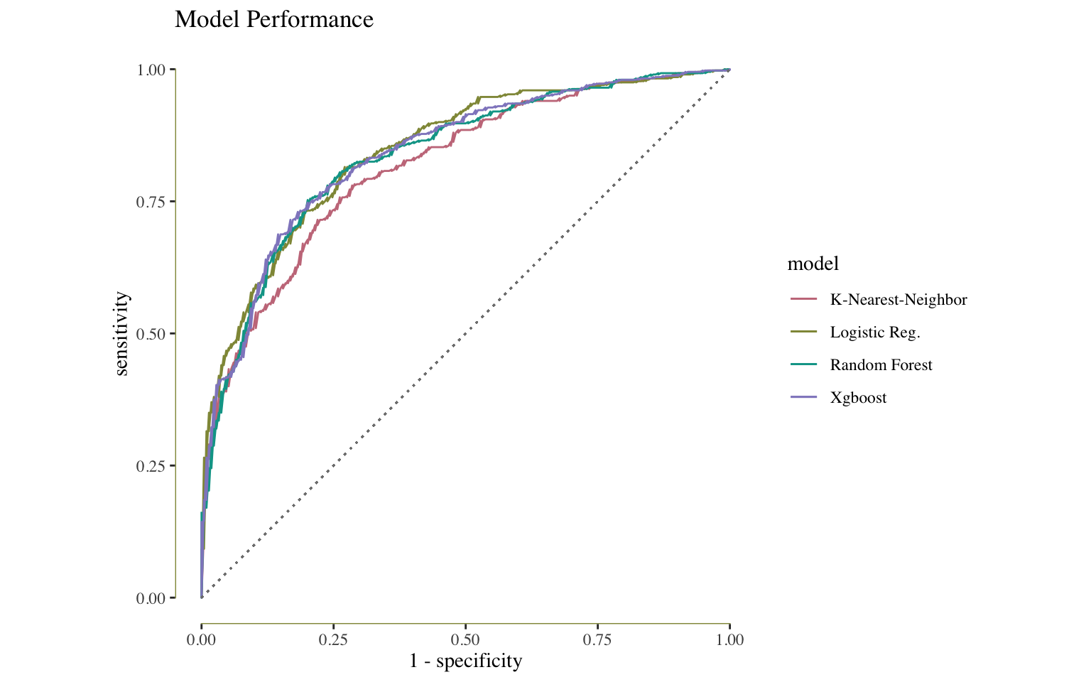
Here, four models are applied to the data and then ranked by area under the curve and accuracy. The four models are logistic regression, k-nearest-neighbor, random forest (ranger) and xgboost. Logistic regression was the best performing when measured by roc_auc (.855) and random forest model was the best performing when measured by accuracy (.772).

Code

#\ label: data-summary
describe(diabetes) |> 
mutate(across(mean:se, ~round(.x, 2))) |> 
kbl() |>
kable_styling(bootstrap_options = c("striped", "hover", "condensed", "responsive"))

	vars	n	mean	sd	median	trimmed	mad	min	max	range	skew	kurtosis	se
pregn	1	768	3.85	3.37	3.00	3.46	2.97	0.00	17.00	17.00	0.90	0.14	0.12
gluco	2	768	123.87	32.86	123.00	122.56	38.55	44.00	199.00	155.00	0.25	-0.58	1.19
bp	3	768	72.21	11.53	72.00	72.19	11.86	24.00	122.00	98.00	0.06	0.67	0.42
skint	4	768	28.96	10.52	28.00	28.59	10.38	7.00	99.00	92.00	0.60	1.84	0.38
insul	5	768	142.48	109.39	115.00	124.84	77.10	14.00	846.00	832.00	2.04	6.05	3.95
bmi	6	768	32.51	7.14	32.60	32.11	7.41	18.20	67.10	48.90	0.68	1.16	0.26
dpf	7	768	0.47	0.33	0.37	0.42	0.25	0.08	2.42	2.34	1.91	5.53	0.01
age	8	768	33.24	11.76	29.00	31.54	10.38	21.00	81.00	60.00	1.13	0.62	0.42
outcome*	9	768	1.35	0.48	1.00	1.31	0.00	1.00	2.00	1.00	0.63	-1.60	0.02

Outliers

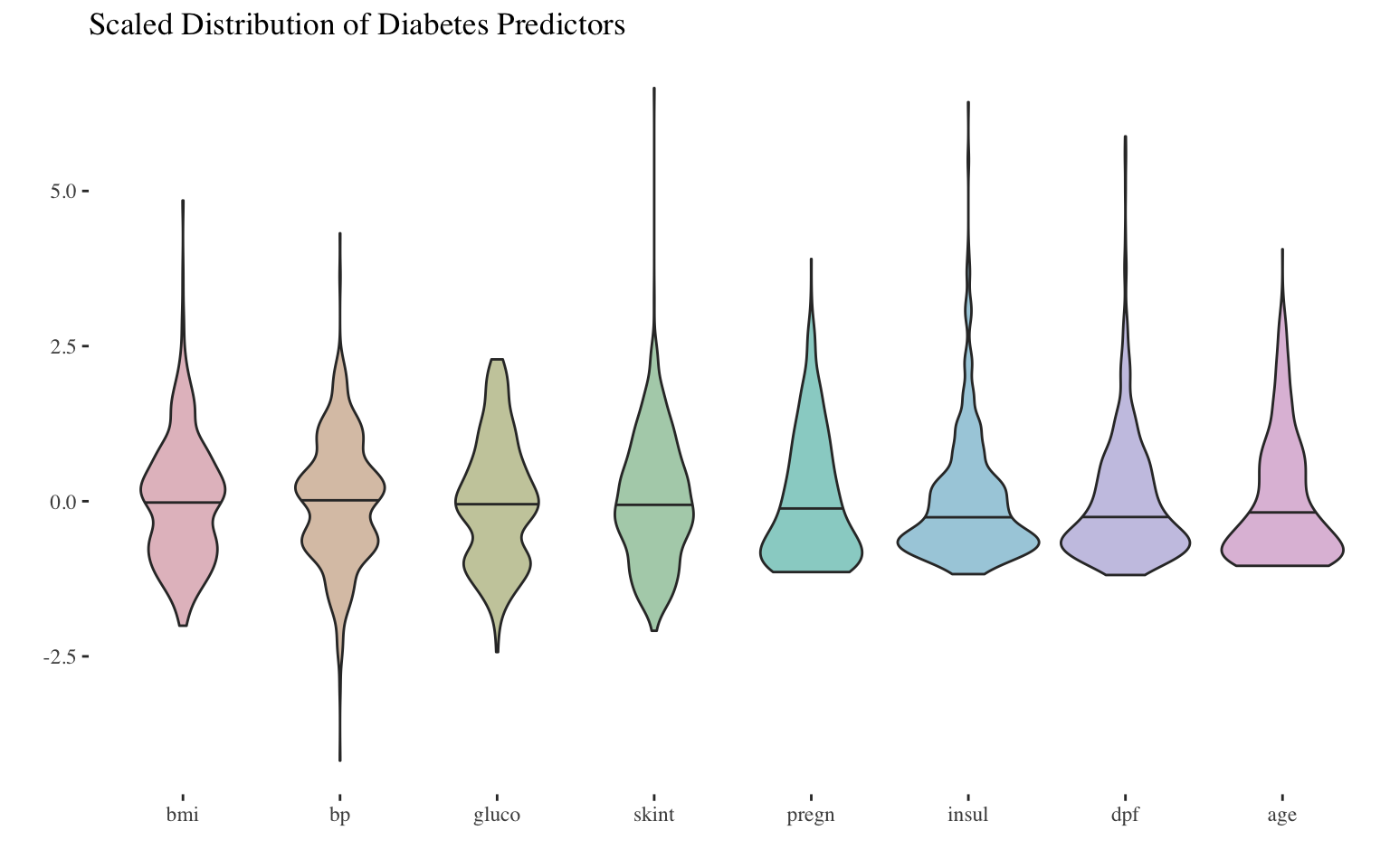
The data set was thoroughly explored on Kaggle. Kagglers report that many values were recorded as a zero. For a category like blood pressure or glucose a “0” would be non-sensical. These values were changed to “NA” and imputed using the mice package. Despite imputation and scaling of the data, many outliers remain as shown below. To repeat once more, the data were scaled.

Code

# plot distributions ----
colors <- qualitative_hcl(n = 8, palette = "Dark2")
diabetes |>
    select(!outcome) |>
    mutate(across(pregn:age, ~scale(.x))) |>
    pivot_longer(pregn:age) |>
    group_by(name) |>
    mutate(median = median(value)) |>
    ungroup() |>
    mutate(name = factor(name)) |>
    mutate(name = forcats::fct_reorder(name, -median)) |>
    ggplot() +
    aes(name, value, group = name, fill = name) +
    geom_violin(alpha = .5, draw_quantiles = c(0.5)) +
    theme_tufte() +
    scale_fill_manual(values = colors) +
    labs(
        title = "Scaled Distribution of Diabetes Predictors",
         x = "",
         y = "") +
    theme(legend.position = "none")

Assessing Model Effectivness

The point of the assignment is to practice the tidy model flow and find the best performing models. Finding the best model means creating an objective measure for evaluation. The diabetes data is a classification problem, but all metrics will be discussed as a reminder for future efforts.

For background, models generally come in two types. “An inferential model is used primarily to understand relationships, and typically emphasizes the choice (and validity) of probabilistic distributions and other generative qualities that define the model.” In predictive models, its strength is more important, i.e. how close its predictions matched the observed data. Silge and Kuhn advise practitioners “developing inferential models . . . to use these techniques even when the model will not be used with the primary goal of prediction.”

The term accuracy is the proportion of the data that are predicted correctly. The Tidy Models book states that “two common metrics for regression models are the root mean squared error (RMSE) and the coefficient of determination (a.k.a. R2). The former measures accuracy while the latter measures correlation A model optimized for RMSE has more variability but has relatively uniform accuracy across the range of the outcome.”

Regression Metrics

metric_set allows for the return of multiple metrics and can be used to return metrics for regression analysis.

regress_metrics <- metric_set(rmse, rsq, mae)

Classification

A classification is usually binary, but it can take on additional classes. A binary classification is where the outcome is one of two possible classes like positive vs. negative or red vs. green. The results often include a probability for each class, like .95 likelihood of occurrence and .05 likelihood of non-occurrence.

For “hard-class” predictions that deal with only the category, not the probability, the yardstick package contains four helpful functions: conf_mat() (confusion matrix), accuracy(), mcc() (Matthew’s Correlation Coefficient), and f_meas(). Three of them could be combined like:

class_metrics <- metric_set(accuracy, mcc, f_meas)

For outcome variables that have multiple classes, the yardstick package contains methods that can be implemented via the “estimator” argument in the sensitivity() function.

# estimator can be "macro_weighted", "macro", "micro"
sensitivity(results, obs, pred, estimator = "macro_weighted")

Confusion Matrix

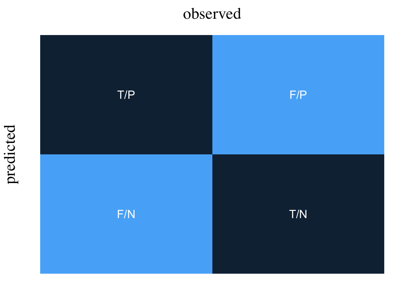
A confusion matrix, also known as an error matrix, reports the performance of a classification model. Where the outcome is one of two classes, the confusion matrix reports the number of observations that were correctly labelled and others that were not. More formally, the confusion matrix is a 2 by 2 table with the following entries:

true positive (TP). A test result that correctly indicates the presence of a condition or characteristic.
true negative (TN). A test result that correctly indicates the absence of a condition or characteristic.
false positive (FP). A test result which wrongly indicates that a particular condition or attribute is present.
false negative (FN). A test result which wrongly indicates that a particular condition or attribute is absent.

Code

dt <- tibble(t = c(1, 2, 1, 2), 
             f = c(1, 2, 2, 1), 
             fill = c(20, 20, 8, 8),
             labels = c("F/N", "F/P", "T/P", "T/N"))
dt |> 
    ggplot() +
    aes(factor(t), factor(f), fill = fill, label = labels) +
    geom_tile() +
    theme_tufte() +
    theme(legend.position = "none",
          axis.ticks = element_blank(),
          axis.title = element_text(size = 20)) +
    scale_x_discrete(name = "observed",
                     labels = NULL,
                     position = "top") +
    scale_y_discrete(name = "predicted",
                     labels = NULL) +
    geom_text(color = "white", size = 5)

Resampling Results

The four models consisted of logistic regression (glmnet), K-nearest-neighbor, Random Forest (ranger), and xgboost.

Code

models <- readRDS("./data/model_performance.rds")
colors <- colorspace::qualitative_hcl(n = 4, palette = "Dark2")
models |>
    ggplot() +
    aes(1 - specificity, sensitivity, color = model) +
    geom_line() +
    geom_segment(x = 0, xend = 1,
                 y = 0, yend = 1,
                 color = "gray50",
                 linetype = 3) +
    coord_equal(ratio = 1) +
    scale_color_manual(values = colors) +
    geom_rangeframe() +
    theme_tufte() +
    labs(title = "Model Performance")

Final Fit on Test Set

Code

results <- readRDS("./data/table_final_results.rds")
results |> 
    kbl(escape = F) |> 
    kable_styling(bootstrap_options = c("striped", "hover", "condensed", "responsive"), full_width = T)

model	.metric	.estimator	.estimate
lr	roc_auc	binary	0.8550000
xgb	roc_auc	binary	0.8396296
rf	roc_auc	binary	0.8305556
knn	roc_auc	binary	0.8122222
rf	accuracy	binary	0.7727273
lr	accuracy	binary	0.7662338
xgb	accuracy	binary	0.7532468
knn	accuracy	binary	0.7142857