Regression Plots

1 Mtcars

2 Regression Model

lm <- lm(mpg ~ hp * wt, data = mtcars)

3 Regression Results

tidy(lm) |>  #broom package
    kbl() |> #kableExtra
    kable_styling(bootstrap_options = c("condensed", "striped"))

term	estimate	std.error	statistic	p.value
(Intercept)	49.8084234	3.6051558	13.815886	0.0000000
hp	-0.1201021	0.0246983	-4.862758	0.0000404
wt	-8.2166243	1.2697081	-6.471270	0.0000005
hp:wt	0.0278481	0.0074196	3.753332	0.0008108

4 Diagnostic Plots

4.1 Default

par(mfrow = c(2, 2))
plot(lm)

4.2 Default Performance Plot

performance::check_model(lm, theme = "see::theme_lucid")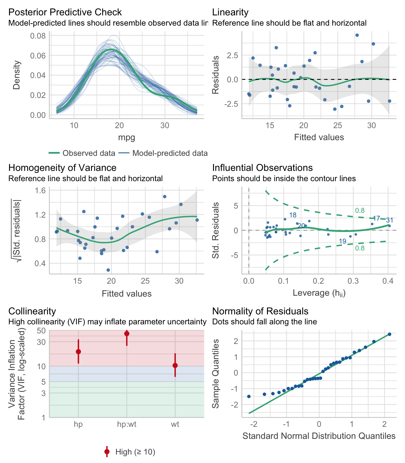

4.3 Theme Minimal

performance::check_model(lm, theme = "ggplot2::theme_minimal")

4.4 Theme Tufte

performance::check_model(lm, theme = "ggthemes::theme_tufte()",
                         colors = c("#C87A8A", "#6B9D59", "#5F96C2"))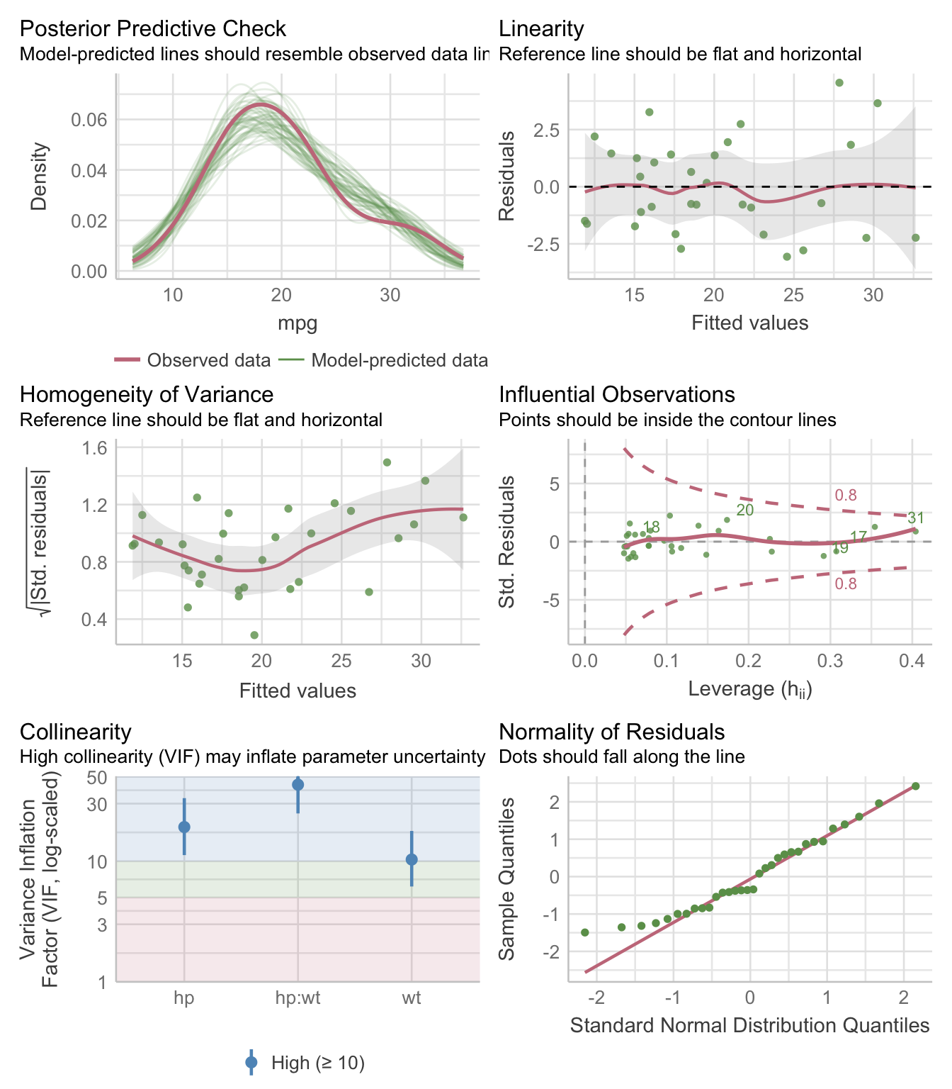

5 Check Normality

check_normality(lm)

OK: residuals appear as normally distributed (p = 0.138).

To better understand the function, run ?performance::check_normality().

6 Check Heteroskedacity

check_heteroskedasticity(lm)

OK: Error variance appears to be homoscedastic (p = 0.055).

To better understand the function, run ?performance::check_heteroskedasticity().

7 Challenges

The themes argument did not work, colors argument did.

8 Acknowledgements

Many thanks to Dr. Lyndon Walker for his tutorial on youtube. His channel can be found here.