Data Structures
1 Objective
The viewer will be able to identify the data structure type (polygon versus multipolygon) and to plot a subset of the data with one of three strategies: (1) filtering, (2) casting, or (3) setting the plot window.
2 Introduction
Many sf datasets will be grouped at the country level. Countries can be a single polygon. However, they are usually comprised of multiple polygons. An example might be the United States, where Hawaii can be found in the middle of the Pacific Ocean. The distance between Hawaii and the mainland U.S. can be problematic because of the amount of space devoted to the surrounding ocean. This scenario occurs frequently. The remainder of the discussion will be devoted to addressing this challenge.
3 Packages Required
Make sure to load the following packages.
4 Distinguish
To mimic the Hawaii-US scenario, two squares will be created, one smaller and one larger. The two squares will go through the familiar sfg-->sfc-->sf pipeline. The polygons will then be placed into two different data structures. Note that if the data are imported via st_read(), the function contains many arguments and all geometries are converted to the “Multi” variety. For example, polygons become multipolygons. In order to keep the original geometries, then the argument promote_to_multi must be set to FALSE.
sq_1 <-
st_polygon(list(rbind(
c(0,0), c(0, 1), c(1, 1), c(1, 0), c(0, 0)
)
)
)
sq_2 <- (sq_1 * 5) + 5
(st_sfc(list(sq_1, sq_2), crs= "WGS84") %>%
st_sf(tibble("name"= c("A", "B")), geometry = .) -> sq_poly)
#> Simple feature collection with 2 features and 1 field
#> Geometry type: POLYGON
#> Dimension: XY
#> Bounding box: xmin: 0 ymin: 0 xmax: 10 ymax: 10
#> Geodetic CRS: WGS 84
#> # A tibble: 2 × 2
#> name geometry
#> <chr> <POLYGON [°]>
#> 1 A ((0 0, 0 1, 1 1, 1 0, 0 0))
#> 2 B ((5 5, 5 10, 10 10, 10 5, 5 5))- 1
-
The operative function is the call to
st_polygon(). - 2
- The next square is a derivative of the first one.
- 3
-
Finally, the squares are placed into a data frame of class
sf.
Note that the geometry type is “POLYGON” and the data frame holds two features.
The two squares created above are recycled in the code below, except that they are placed as a single multipolygon.
(st_multipolygon(list(sq_1, sq_2)) %>%
st_sfc(., crs = "WGS84") %>%
st_sf(tibble("name" = c("A")), geometry = .) -> sq_mpoly)
#> Simple feature collection with 1 feature and 1 field
#> Geometry type: MULTIPOLYGON
#> Dimension: XY
#> Bounding box: xmin: 0 ymin: 0 xmax: 10 ymax: 10
#> Geodetic CRS: WGS 84
#> # A tibble: 1 × 2
#> name geometry
#> <chr> <MULTIPOLYGON [°]>
#> 1 A (((0 0, 0 1, 1 1, 1 0, 0 0)), ((5 5, 5 10, 10 10, 10 5, 5 5)))- 1
-
The operative function is
st_multipolygon(). - 2
- Since the creation only results in one line, only a single name “A” is assigned.
Note that the geometry type produced is “MULTIPOLYGON” and the data frame holds one feature.
p1 <-
    sq_poly %>%
    ggplot() +
    geom_sf(fill = "steelblue") +
    coord_sf() +
    theme_bw() +
    labs(title = "st_polygon()")
p2 <-
    sq_mpoly %>%
    ggplot() +
    geom_sf(fill = "steelblue") +
    coord_sf() +
    theme_bw() +
    labs(title = "st_multipolygon()")
p1 + p2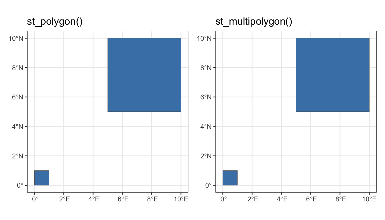
It is crucial in developing a plotting strategy to understand the underlying data structure. If you want to plot a portion of the data, there are several strategies available, but the first step will always be in understanding how the features are stored.
5 Three Ways to Plot
There are at least three ways to plot the data such that only one polygon is in the plot.
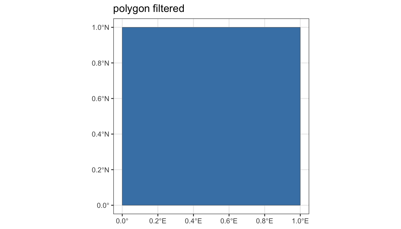
5.1 Filter
If the data structure is a data frame of two simple features and those features are polygons, then the data structure may be filtered to the chosen polygon using the familiar dplyr pipe. Below polygon “A” was chosen but polygon “B” could have been chosen as well.
5.2 Cast
If you wish to subset a multipolygon object, it may be necessary to separate out the individual polygons. The function to inspect each polygon is st_cast().
st_cast(sq_mpoly, to = "POLYGON")
#> Simple feature collection with 2 features and 1 field
#> Geometry type: POLYGON
#> Dimension:     XY
#> Bounding box:  xmin: 0 ymin: 0 xmax: 10 ymax: 10
#> Geodetic CRS:  WGS 84
#> # A tibble: 2 × 2
#>   name                         geometry
#>   <chr>                   <POLYGON [°]>
#> 1 A         ((0 0, 0 1, 1 1, 1 0, 0 0))
#> 2 A     ((5 5, 5 10, 10 10, 10 5, 5 5))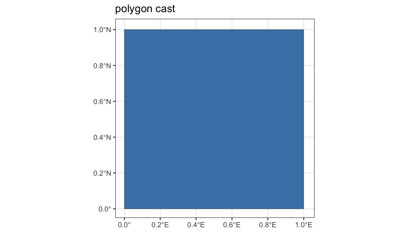
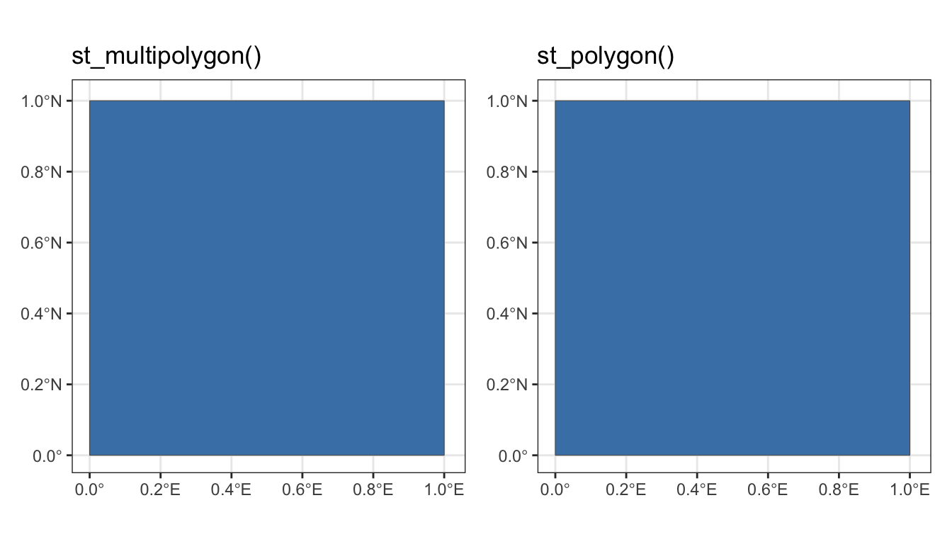
5.3 Set Window
p1 <-
sq_mpoly %>%
ggplot() +
geom_sf(fill = "steelblue") +
coord_sf(xlim = c(0, 1.01), ylim = c(0, 1.01)) +
theme_bw() +
labs(title = "st_multipolygon()")
p2 <-
sq_poly %>%
ggplot() +
geom_sf(fill = "steelblue") +
coord_sf(xlim = c(0, 1.01), ylim = c(0, 1.01)) +
theme_bw() +
labs(title= "st_polygon()")
p1 + p2- 1
- Operative code for setting the range.
- 2
- Operative code for seeting the range.
6 Hawaii Example
After importing a dataset and performing an initial plot, there is often some unexpected geometries. Here, the U.S. states will be imported from the rnaturalearth package. And like usual, when the target (here Hawaii) is inspected, there’s some surprising results.
According to the Department of State, the Hawaiian Islands were first discovered by the West in 1778 by Captain James Cook. Cook named the islands the “Sandwich Islands” after the British Earl of Sandwich. Having become a territory in 1898, Hawaii became a state in 1959. (U.S. Dept. of State, 2024) According to Wikipedia, “the Hawaiian Island archipelago extends some 1,500 miles (2,400 km) from the southernmost island of Hawaiʻi to the northernmost Kure Atoll.”
(us <- rnaturalearth::ne_states(country = "United States of America") %>%
    dplyr::select(postal, geometry))
#> Simple feature collection with 51 features and 1 field
#> Geometry type: MULTIPOLYGON
#> Dimension:     XY
#> Bounding box:  xmin: -179 ymin: 18.9 xmax: 180 ymax: 71.4
#> Geodetic CRS:  WGS 84
#> First 10 features:
#>      postal                       geometry
#> 1236     WA MULTIPOLYGON (((-123 49, -1...
#> 1238     ID MULTIPOLYGON (((-117 49, -1...
#> 1239     MT MULTIPOLYGON (((-116 49, -1...
#> 1242     ND MULTIPOLYGON (((-104 49, -1...
#> 1244     MN MULTIPOLYGON (((-97.2 49, -...
#> 1246     MI MULTIPOLYGON (((-84.5 46.5,...
#> 1247     OH MULTIPOLYGON (((-80.5 42, -...
#> 1248     PA MULTIPOLYGON (((-79.8 42.3,...
#> 1249     NY MULTIPOLYGON (((-79.1 43.1,...
#> 1251     VT MULTIPOLYGON (((-73.4 45, -...
Results in a sf class data frame with 51 features and a geometry type of “MULTIPOLYGON”.
6.1 Filter
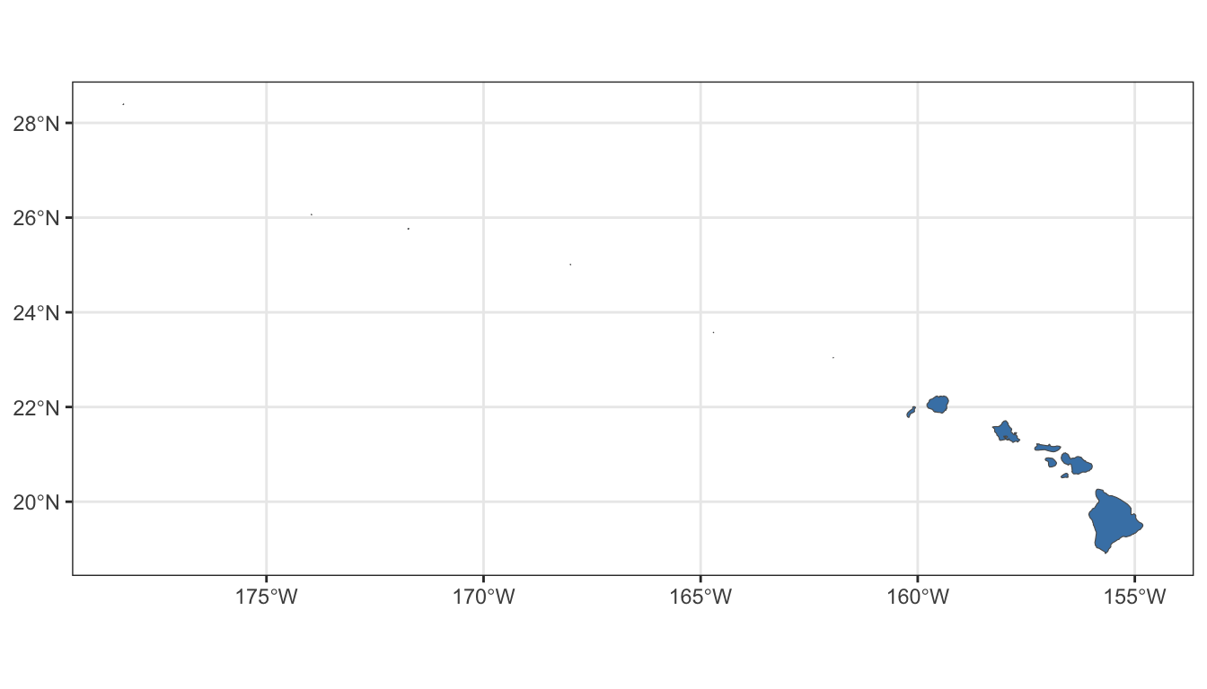
Using the method described above, the sf class data frame is filtered to Hawaii and plotted.
6.2 Cast
After some investigation, Hawaii is actually comprised of 14 separate islands. In order to see the individual polygons, they will have to be extracted from the “MULTIPOLYGON” geometry and inspected. This is the role of the st_cast() function.
hi <- us %>% dplyr::filter(postal == "HI")
(hi_cast <- sf::st_cast(hi, to = "POLYGON"))
#> Simple feature collection with 14 features and 1 field
#> Geometry type: POLYGON
#> Dimension:     XY
#> Bounding box:  xmin: -178 ymin: 18.9 xmax: -155 ymax: 28.4
#> Geodetic CRS:  WGS 84
#> First 10 features:
#>     postal                       geometry
#> 1       HI POLYGON ((-155 19.6, -155 1...
#> 1.1     HI POLYGON ((-157 20.6, -157 2...
#> 1.2     HI POLYGON ((-157 20.9, -157 2...
#> 1.3     HI POLYGON ((-156 20.8, -156 2...
#> 1.4     HI POLYGON ((-157 21.2, -157 2...
#> 1.5     HI POLYGON ((-158 21.4, -158 2...
#> 1.6     HI POLYGON ((-160 22, -160 22,...
#> 1.7     HI POLYGON ((-159 22.2, -159 2...
#> 1.8     HI POLYGON ((-162 23, -162 23,...
#> 1.9     HI POLYGON ((-165 23.6, -165 2...
Now that the individual polygons can be inspected, we’re going to create a column for the area of each island. The working hypothesis is that around 6 of the islands are so small that they are invisible on the plotting panel. Because of that, we’ll also create a label/text column. The islands could have been labeled based on size, but I decided to label them from left to right using longitude. The code to create the new columns is below.
hi_all %>%
    ggplot() +
    geom_sf(fill = "steelblue") +
    geom_text_repel(
        data = hi_all,
        mapping = aes(x = lon, y = lat, label = island)) +
    coord_sf() +
    theme_bw()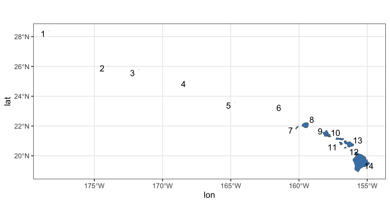
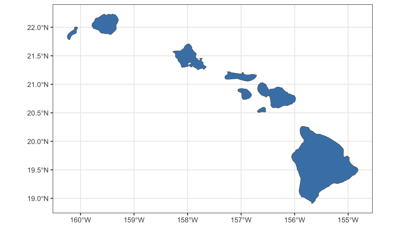
With the labels visible, it is clear that the original plot was correct and the bounding box was sized appropriately. With visual confirmation, the islands will be subset to the largest islands using longitude or label.
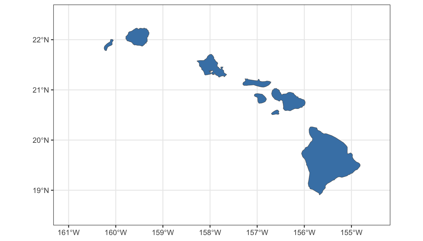
6.3 Set Window
The final strategy to plotting Hawaii is to simply adjust the plotting area range.
7 Key Points
Plotting effectively requires an understanding of the underlying data structure.
Upon import,
sfclass data frames will default to “MULTIPOLYGON”.“MULTIPOLYGON” may mean there is only one contiguous polygon, although most countries and states will be comprised of more than one.
Plotting an area of interest and relevance may require subsetting polygons.
There are at least three strategies for subsetting a
sfclass data frame for plotting: (1) filtering the dataset, (2) casting the dataset, or (3) adjusting the plotting window.