Text and Labels

1 Objective

The objective for this section is to learn how to label map features with either labels or text.

2 Introduction

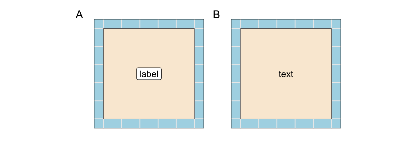
Unless a viewer is personally familiar with a map’s content, textual descriptions will be necessary. “Text” and “label” are terms of art and have specific meaning within the R-spatial packages. A “label” is text placed on a background with a border. The addition of a background can bring greater contrast and attract the attention of the viewer. “Text” is just basic text without any background.

Figure 1: Plot “A” is an example of a label while Plot “B” is an example of text.

Within ggplot2, the operative functions are geom_sf_label() and geom_sf_text(). The functions can be helpful when the data has a small number of observations. However, a more helpful approach is theggrepel package which uses an algorithm to separate the text labels. This can save a cartographer a lot of manual work in label placement. The two functions are geom_text_repel() and geom_label_repel(). The labels and text will repel from one another and the sides of the plot. While the algorithm can be helpful for a moderate number of points, it may be overwhelmed with large numbers.

3 Packages Required

library(colorspace)
library(dplyr)
library(ggplot2)
library(ggrepel)
library(magrittr)
library(sfheaders)
library(sf)
library(tibble)
library(tidyr)
library(tmap)

4 Functions

The function below creates 25 random squares on a map. Knowledge of its details are unnecessary and, therefore, the code block was hidden.

4.1 Polygons

Code

create_polys <- function(n_obs = 5, side_length = 5){
    lat_range <- seq(-85, 85, by = 5)
    lng_range <- seq(-175, 175, by = 5)
    y_origin <- sample(lat_range, n_obs, replace = F)
    x_origin <- sample(lng_range, n_obs, replace = F)
    df <- tibble()
    for(i in 1:length(x_origin)){
        p <-
            tibble(
                id = i,
                x_1 = x_origin[i],
                y_1 = y_origin[i],
                x_2 = x_origin[i],
                y_2 = y_origin[i] + side_length,
                x_3 = x_origin[i] + side_length,
                y_3 = y_origin[i] + side_length,
                x_4 = x_origin[i] + side_length,
                y_4 = y_origin[i],
                x_5 = x_origin[i],
                y_5 = y_origin[i]
                )
        p_xy <-
            p |>
            pivot_longer(cols = x_1:y_5) |>
            separate(name, into = c("axis", "call"), sep = "_") |>
            select(id, call, everything()) |>
            pivot_wider(names_from = axis, values_from = value) |>
            select(-call)
        df <- dplyr::bind_rows(df, p_xy)
    }

    sf <- sfheaders::sf_polygon(
        obj = df,
        , x = "x"
        , y = "y"
        , polygon_id = "id"
    )
    sf::st_crs(sf) <- "WGS84"
    sf$var_cont <- rnorm(n_obs)
    sf$var_fact <- ggplot2::cut_interval(sf$var_cont, n = 5, labels = c(letters[1:5]))
    sf$id <- as.character(sf$id)
    sf
}
polys <- create_polys(n_obs = 25)

4.2 Polygon Centers

Usually in labeling, “point” data is necessary to anchor the label to the plot. This can be accomplished by the sf::st_centroid() function. The code block below is used ad nauseum for this purpose.

poly_ctr <-
    polys %>%
    sf::st_centroid() %>%
    dplyr::mutate(lon = sf::st_coordinates(.)[, 1],
                  lat = sf::st_coordinates(.)[, 2])

5 Square Land

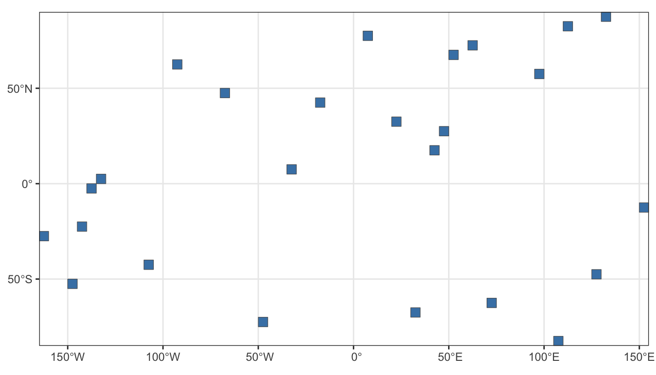
5.1 Base Layer

The base layer was generated using the polygon function. The function creates random, same-sized squares on a “WGS 84” plotting grid where latitude is from -90 to 90 and longitude is -180 to 180. The first plot is just to show the base features.

ggplot() +
    geom_sf(data = polys, fill = "steelblue") +
    coord_sf(expand = F) +
    theme_bw()

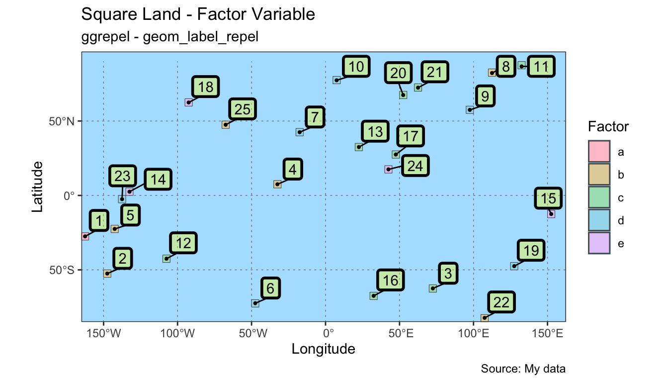
5.2 Labels - Factor

The first plot is with data where one column is a factor variable; the annotation is a label; and the colors are from a colorspace qualitative HCL palette named “Pastel 1”. Some arguments to the geom_label_repel() function were chosen to illustrate functionality.

colors <- qualitative_hcl(n = 5, palette = "pastel1")
ggplot() +
geom_sf(data = polys, mapping = aes(fill = var_fact), 
        show.legend = T) +
scale_fill_manual("Factor", values = colors) +
geom_sf(data = poly_ctr, size = .75, show.legend = F) +
geom_label_repel(data = poly_ctr,
                aes(x = lon, y = lat, label = id),
                fill = alpha("yellow", .35),
                nudge_y = 10,
                nudge_x = 10,
                min.segment.length = 0,
                label.size = 1
)  +
coord_sf(expand = F) +
theme_bw() +
theme(
    panel.grid.major = element_line(
        color = gray(.5),
        linetype = "dotted",
        linewidth = 0.25
        ),
    panel.background = element_rect(
        fill = "lightskyblue1"
        )
) +
labs(title = "Square Land - Factor Variable",
     subtitle = "ggrepel - geom_label_repel",
     caption = "Source: My data") +
xlab("Longitude") +
ylab("Latitude")

1: Operative lines for the geom_label_repel() function.

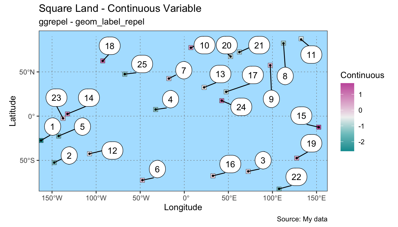
Figure 3: Plot of random squares with labels. Note how the repel algorithm moves the labels. The plotted factor variable has 5 categories.

5.3 Labels - Continuous

The second plot is with data where a second column is a continuous variable; the annotation is a label; and the colors are from colorspace diverging HCL palette named “Tropic”.

colors <- diverge_hcl(n = 5, palette = "tropic") 
ggplot() +
geom_sf(data = polys, mapping = aes(fill = var_cont),  
        show.legend = T) + 
scale_fill_gradientn("Continuous", colours = colors) + 
geom_sf(data = poly_ctr, size = .75, show.legend = F) +
geom_label_repel(data = poly_ctr,
                 aes(x = lon, y = lat, label = id),
                 nudge_y = 10,
                 nudge_x = 10,
                 min.segment.length = 0,
                 box.padding = .5,
                 label.padding = .5,
                 label.r = .75
) +
coord_sf(expand = F) +
theme_bw() +
theme(
    panel.grid.major = element_line(
        color = gray(.5),
        linetype = "dotted",
        linewidth = 0.25
    ),
    panel.background = element_rect(
        fill = "lightskyblue1"
    )
) +
labs(title = "Square Land - Continuous Variable",
     subtitle = "ggrepel - geom_label_repel",
     caption = "Source: My data") +
xlab("Longitude") +
ylab("Latitude")

1: Operative code lines for geom_label_repel().

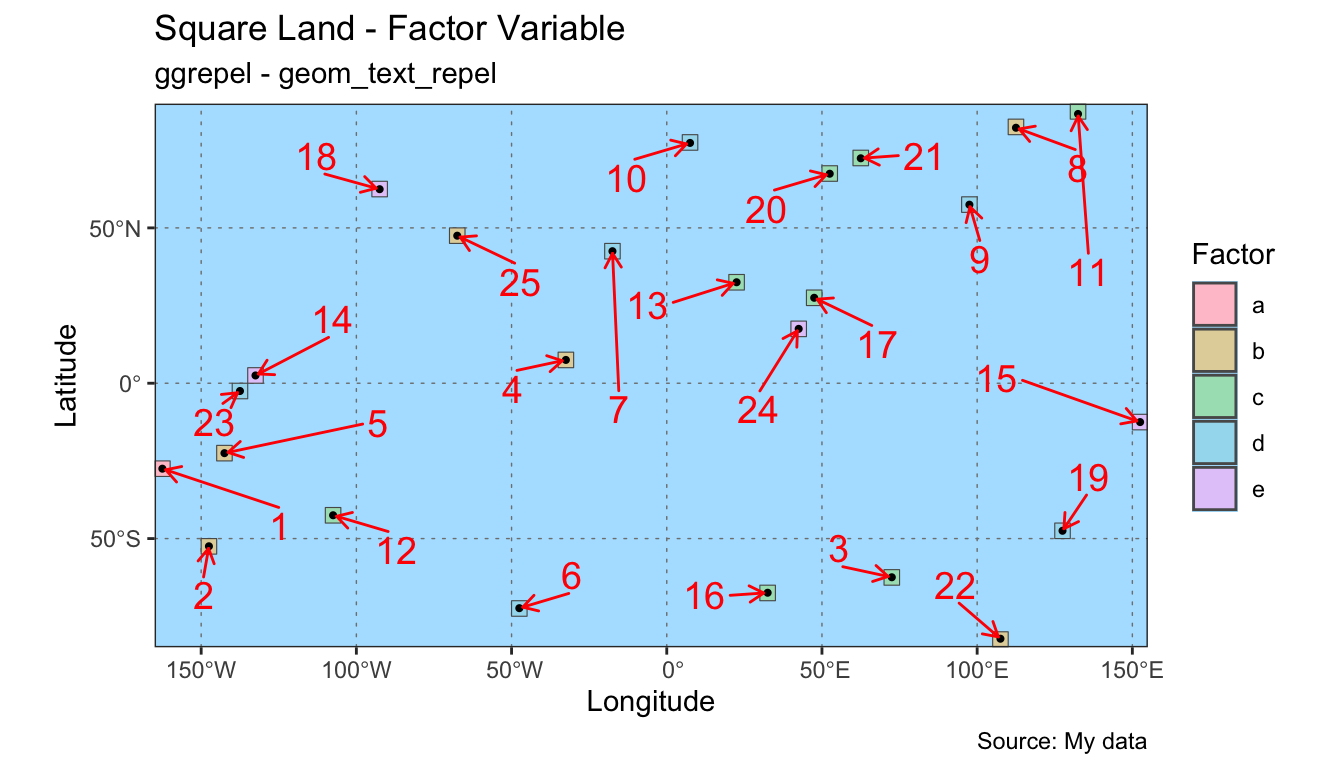
Figure 4: Plot of random squares with labels. Note how the repel alogrithm moves some of the labels. A diverging color palette was chosen to emphasize the outliers in both tails of the distribution.

5.4 Text - Factor

The third plot is with data where a column is a factor variable; the annotation is text; and the colors are from colorspace qualitative HCL palette named “Pastel 1”. Because of the switch from label to text, there are fewer options for the styling of the annotation. However, the line segment can be styled and an arrow head added.

colors <- colorspace::qualitative_hcl(n = 5, palette = "pastel1")
ggplot() +
geom_sf(data = polys, mapping = aes(fill = var_fact), show.legend = T) +
scale_fill_manual("Factor", values = colors) +
geom_sf(data = poly_ctr, size = .75, show.legend = F) +
geom_text_repel(data = poly_ctr,
                 aes(x = lon, y = lat, label = id),
                 nudge_y = 0,
                 nudge_x = 0,
                 min.segment.length = 0,
                 color = "red",
                 box.padding = 1,
                arrow = arrow(length = unit(0.03, "npc"),
                              type = "open"),
                 size = 5
) +
coord_sf(expand = F) +
theme_bw() +
theme(
    panel.grid.major = element_line(
        color = gray(.5),
        linetype = "dotted",
        linewidth = 0.25
    ),
    panel.background = element_rect(
        fill = "lightskyblue1"
    )
) +
labs(title = "Square Land - Factor Variable",
     subtitle = "ggrepel - geom_text_repel",
     caption = "Source: My data") +
xlab("Longitude") +
ylab("Latitude")

1: Operative code lines for geom_text_repel().

Figure 5: Plot of random squares with text as annotation.

5.5 Text - Continuous

The fourth plot is with data where a column is a continuous variable; the annotation is text; and the colors are from colorspace diverging HCL palette named “Green-Orange”.

colors <- diverge_hcl(n = 5, palette = "green-orange")
ggplot() +
geom_sf(data = polys, mapping = aes(fill = var_cont), 
        show.legend = T) +
scale_fill_gradientn("Continuous", colours = colors) +
geom_sf(data = poly_ctr, size = .75, show.legend = F) +
geom_text_repel(data = poly_ctr,
                 mapping = aes(x = lon, y = lat, 
                     label = id, size = var_cont),
                 nudge_y = 10,
                 nudge_x = 10,
                 min.segment.length = 0,
                show.legend = F
) +
coord_sf(expand = F) +
theme_bw() +
theme(
    panel.grid.major = element_line(
        color = gray(.5),
        linetype = "dotted",
        linewidth = 0.25
    ),
    panel.background = element_rect(
        fill = "lightskyblue1"
    )
) +
labs(title = "Square Land - Continuous Variable",
     subtitle = "ggrepel - geom_text_repel",
     caption = "Source: My data") +
xlab("Longitude") +
ylab("Latitude")

1: Operative code lines for geom_text_repel(). Note that a variable is being mapped to the size attribute for the text.

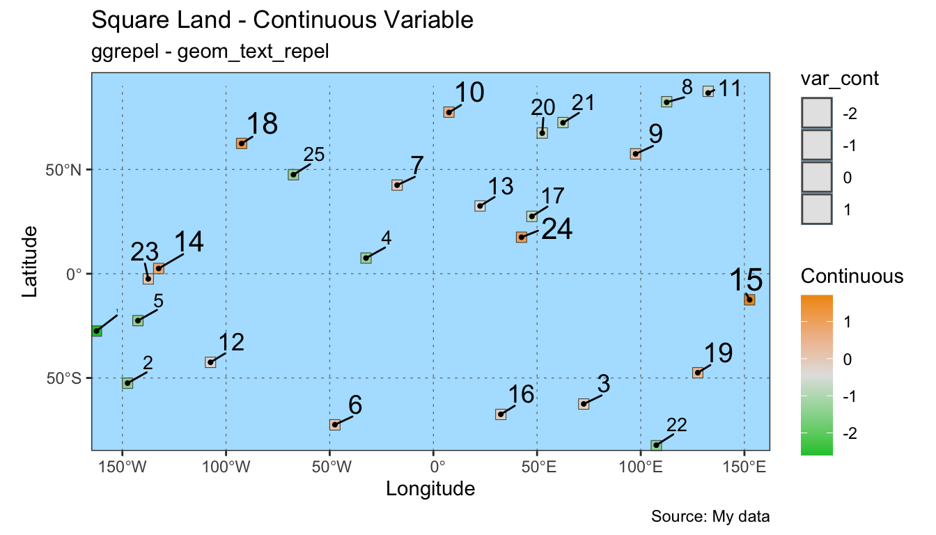
Figure 6: Plot of random squares with text as annotation. Note that the column `var_cont` is being mapped to the size attribute. Large numbers result in larger font sizes.

6 Key Points

The ggrepel package allows labels to be spaced algorithmically rather than manually. This can save time and improve map appearance.
The geom_label_repel and geom_text_repel have many arguments that allow for flexibility in the customization of plots.