Base Plots

1 Objectives

The objective for this section is to quickly and confidently use base plots for verifying data by:

• finding the class of a spatial object

• knowing how to find help when plotting

• understanding how to layer plots

• arranging multiple plots on the same grid

• adjusting a plot’s margins

2 Introduction

I’ll have to admit that I rarely use the base plot method, but instead default to ggplot2 for all static plots. However, with GIS data, it’s a necessity to do quick checks and the plot function makes it so easy. The sf package includes a vignette on the topic, vignette(package = "sf", "sf5") and it should be the starting point for learning about plotting (Pebesma & Bivand, 2023). However, there’s some key points that should be bolstered so you can take full advantage of the base plot functionality.

Base vs. Graphics

From the generic x-y plotting help: “The plot generic was moved from the graphics package to the base package in R 4.0.0. It is currently re-exported from the graphics namespace to allow packages importing it from there to continue working, but this may change in future versions of R.” Any references to the “base” plot is either a reference to the first layer of the map or a rudimentary plot regardless of where it is technically housed.

3 Packages Required

Make sure to load the following packages.

library(magrittr)
library(rnaturalearth)
library(sf)
library(withr)

4 Interpreting the “Help” page

If you run ?sf::plot.sf, the help page will appear. So long as you have the sf package loaded and the object you’re plotting is of class sf, you shouldn’t have any problems. The first thing to notice is that the help page is long and the function arguments depend on the class of the object plotted. For example, when a point is created, it has a class assigned.

sf::st_point(c(0, 1)) %>% class()
#> [1] "XY"    "POINT" "sfg"

The “sfg” above tells you where to look on the help page. You should be looking for the section marked as “## S3 method for class ‘sfg’”. The arguments listed there are options available for the plot. The “sfg” class is usually the first step in the progression of an object becoming an “sf” class object. And most GIS datasets that are imported will have the “sf” class assigned. For that reason, I’ve included a screenshot of the help page for the “## S3 method for class sf”.

Figure 1: Screenshot of the plotting help page and the ellipses within the function arguments.

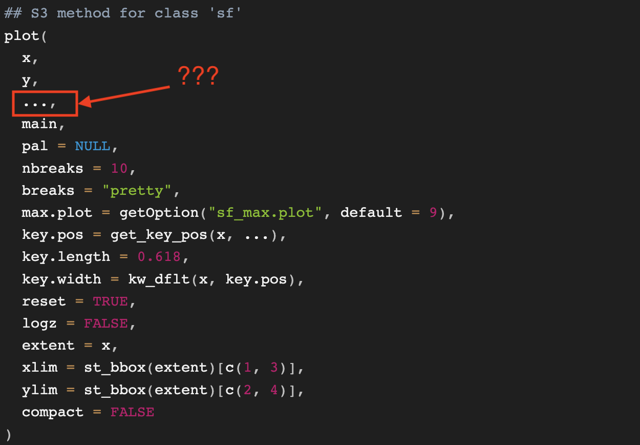
All of the arguments listed are available for customization. However, the innocuous little ellipsis ... creates so many more opportunities! The ellipsis is why this section is a necessity.

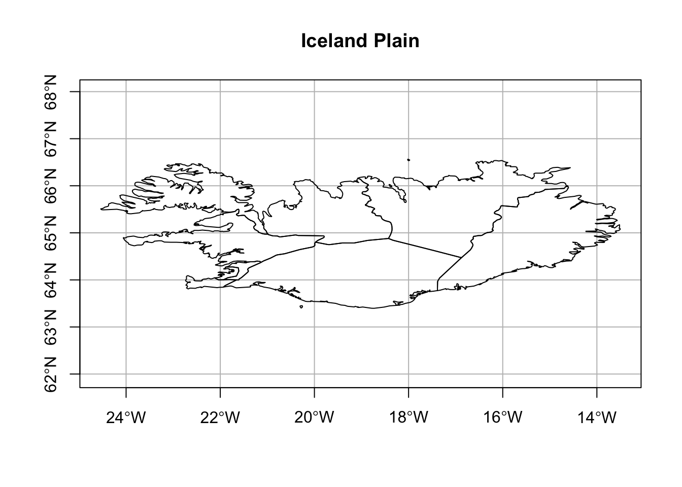
5 Iceland - Plain

Let’s start with a plot of Iceland. The important part is to understand how the geometry column is named. In the dataset from rnaturalearth, the column name is “geometry” and it is a class of sf. Iceland is just south of the Artic circle but has a temperate climate due to the Gulf Stream. Home to 380,000 Icelanders, there are 9 regions.

iceland <- rnaturalearth::ne_states(country = "Iceland") %>% 
    dplyr::select(name, geometry) %>% print(n = 5)
#> Simple feature collection with 9 features and 1 field
#> Geometry type: MULTIPOLYGON
#> Dimension:     XY
#> Bounding box:  xmin: -24.5 ymin: 63.4 xmax: -13.5 ymax: 66.6
#> Geodetic CRS:  WGS 84
#> First 5 features:
#>                  name                       geometry
#> 2356       Austurland MULTIPOLYGON (((-14.6 66, -...
#> 2357        Suðurland MULTIPOLYGON (((-17.4 63.8,...
#> 2358         Suðurnes MULTIPOLYGON (((-21.9 63.8,...
#> 2359        Reykjavík MULTIPOLYGON (((-22.1 64, -...
#> 2360 Höfuðborgarsvæði MULTIPOLYGON (((-21.9 64.3,...
class(iceland)
#> [1] "sf"         "data.frame"

Both of those inquiries are confirmed. Next, Iceland will be plot using the graphics and sf packages. This code proceeds in three steps: it (1) calls the graphics device, (2) plots Iceland, and (3) turns the graphics device off.

png(filename = here::here("images/plotting_intro_iceland.jpg"),
     width = 6,
     height = 6,
     units = "in",
     pointsize = 9,
     bg = NA,
    res = 300
    )
# plot
plot( 
    st_geometry(iceland),
    main = "Iceland Plain",
    axes = T
)
dev.off()

1

Set up to save plot. PNG was used to illustrate transparency. JPG is another option.

2

bg = NA causes the plot background to be transparent.

3

The res setting is a tradeoff between clarity and file size.

4

st_geometry works and so does iceland$geometry.

5

axes = T was not described in the sf::plot help. This simple addition adds a neat line and axis labels.

6

Turning off the graphics device causes the plotting parameters to be reset to initial defaults. Failing to turn the graphics device off can result in unexplained code behavior.

Figure 2: Iceland plotted from a simple, easy command.

Saved Plots vs. Viewer Window

Saved plots often differ in significant ways from a plot that was in the viewer. Frequent comparisons are required to correctly set the parameters.

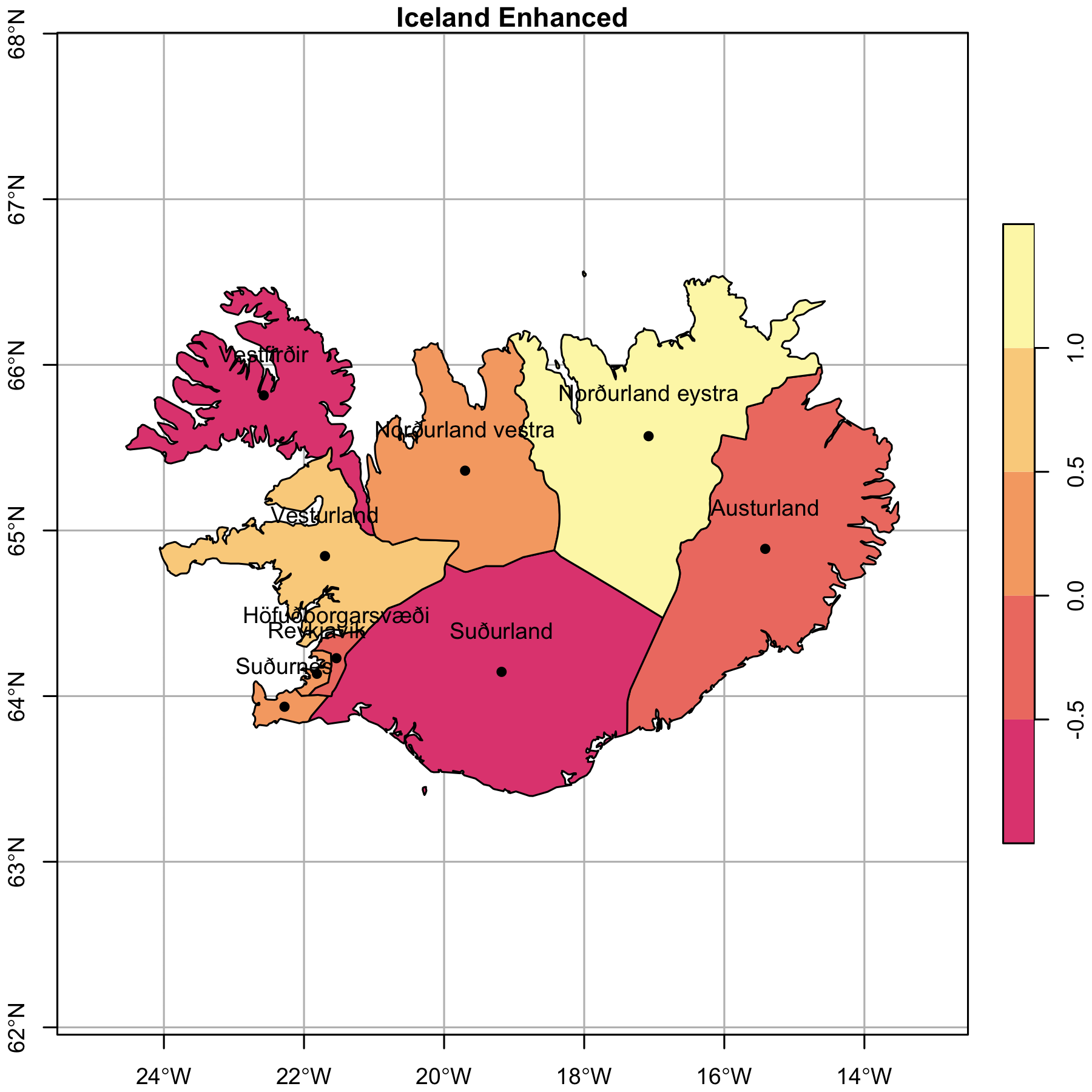
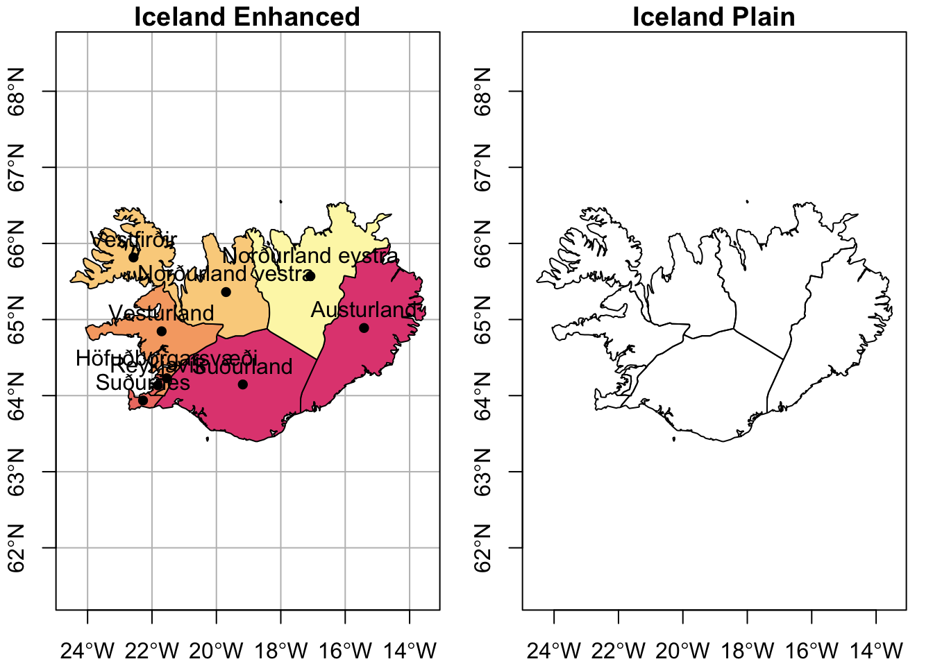
6 Iceland - Enhanced

The plain Iceland above is fine. The plot showed that the geometries are in tact and its coordinates with very little effort. But are there additions can be made to enhance the usability and aesthetics? This time we’ll add several new layers: Iceland, Iceland’s region centroids, and region names, a graticule, and a legend.

library(sf)
rnaturalearth::ne_states(country = "Iceland") %>% 
dplyr::select(name, geometry) %>% 
dplyr::mutate(var_cont = 1:9) -> iceland

iceland %>% 
st_geometry() %>% 
st_centroid() -> region_cntr

st_geometry(iceland) %>% 
st_centroid() %>% 
st_coordinates() %>% 
tibble::as_tibble() %>% 
dplyr::bind_cols(iceland["name"]) %>% 
st_drop_geometry() %>% 
dplyr::rename(lng = "X", lat = "Y") -> region_names

1

First layer is Iceland’s geometry and region names.

2

Second layer is the center of the different regions.

3

Third layer is the names of the regions.

Like above, we’ll plot the enhanced map of Iceland.

png(filename = here::here("images/plotting_intro_iceland_enhanced.png"),
    height = 6,
    width = 6,
    units = "in",
    pointsize = 9,
    bg = NA,
    res = 300
)
plot(
    iceland["var_cont"],
    main = "Iceland Enhanced",
    axes = T,
    graticule = T,
    reset = F,
    border = "black",
    key.pos = 4,
    extent = c(st_bbox(iceland) + c(-.5, -.5, .5, .5)),
    nbreaks = 5,
    pal = colorspace::sequential_hcl(n = 5, palette = "PinkYl")
)
plot(region_cntr, add = T, pch = 16)
text(region_names$lng, region_names$lat + .25, region_names$name)
dev.off()

1

Same configuration as the plot above with the exception of the filename.

2

Big difference between plotting the geometry and an attribute column. A continuous variable column with numbers 1-9 was added.

3

Make sure this is set to “FALSE” if you’re going to add additional layers.

4

The extent argument did not have much in the way of documentation. The bounding box was extended one half of one degree in each direction.

5

I tend to use the colorspace package to generate palettes, but there’s lots of good choices–RColorBrewer is certainly a good one.

6

One-quarter degree was added to the latitude coordinate so the text would be above the centroid point.

Figure 3: Illustration of maximizing base plot arguments to produce a better quality map.

7 withr Package

Using the base plotting method will require, perhaps not immediately, some understanding of the parameters of the graphing device and its defaults. The parameters are accessed via the par function and there’s a bunch of them. We’ll discuss only two here: the mfrow and mai functions. But before explaining their usefulness, we’re going to take a slight diversion to the withr package and the with_par() function.

A big problem occurs when a programmer changes a global default, but then forgets to change it back. For a detailed explanation, on why it’s dangerous to change the programming landscape, see vignette("changing-and-restoring-state", package = "withr") (hester_withr_2024?). This can be diffcult to replicate as knitr opens a new device for each code chunk. In the following sections, we’ll be changing some global defaults to the graphing package. In order to do it in a programatically smart way, we’ll use the with_par() function. The plots will be wrapped in the function and the syntax may look odd.

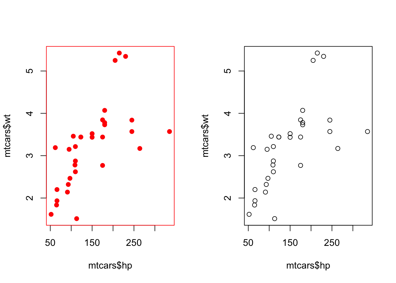
7.1 Poor Way

par()$col
par(col = "red")
par()$col
#> [1] "black"
#> [1] "red"

1

See the current parameter setting for the default color.

2

Set default plotting color to “red”.

3

See if parameter setting changed.

par(mfrow = c(1, 2))
par(col = "red")
plot(mtcars$hp, mtcars$wt)
plot(mtcars$hp, mtcars$wt)

1

Color parameter is not reset between plots, but persists.

Figure 4: Side-by-side comparison showing the persistence of the red color parameter across plots.

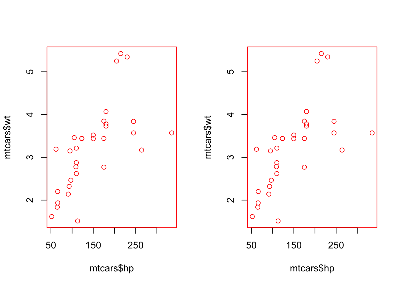
7.2 Better Way

par(mfrow = c(1, 2))
# This will be in red
with_par(list(col = "red", pch = 19),
  plot(mtcars$hp, mtcars$wt)
)
# This will still be in black
plot(mtcars$hp, mtcars$wt)

par()$col

#> [1] "black"

1

Parameter change lasts only within the environment of the with_par function.

Figure 5: Side-by-side comparison of plots showing the color parameter as temporary.

Working within a code chunk presents a different challenge than the normal programming environment. Good practice is use the withr package when changing par arguments from their default value.

8 Multiple Plots

When plotting in the base environment, you may want to have multiple plots. This can be helpful when you want a side-by-side comparison, like “before” and “after” plots. When you want to populate by row, you use mfrow and, when you want to populate by column, you use mfcol.

par(mfrow = c(1, 2))
plot(
    iceland["var_cont"], 
    main = "Iceland Enhanced",
    axes = T,
    graticule = T,
    reset = F,  
    border = "black",
    key.pos = NULL,
    extent = c(st_bbox(iceland) + c(0, 0, 0, 0)),
    nbreaks = 5,
    pal = colorspace::sequential_hcl(n = 5, palette = "PinkYl") 
)
plot(region_cntr, add = T, pch = 16)
text(region_names$lng, region_names$lat + .25, region_names$name)

plot( 
    st_geometry(iceland), 
    main = "Iceland Plain",
    axes = T
)

1

Legend was omitted

2

Buffer for bounding box was omitted

Figure 6: Side-by-side comparison of Iceland Enhanced with robust use of options and Iceland Plain with minimal options.

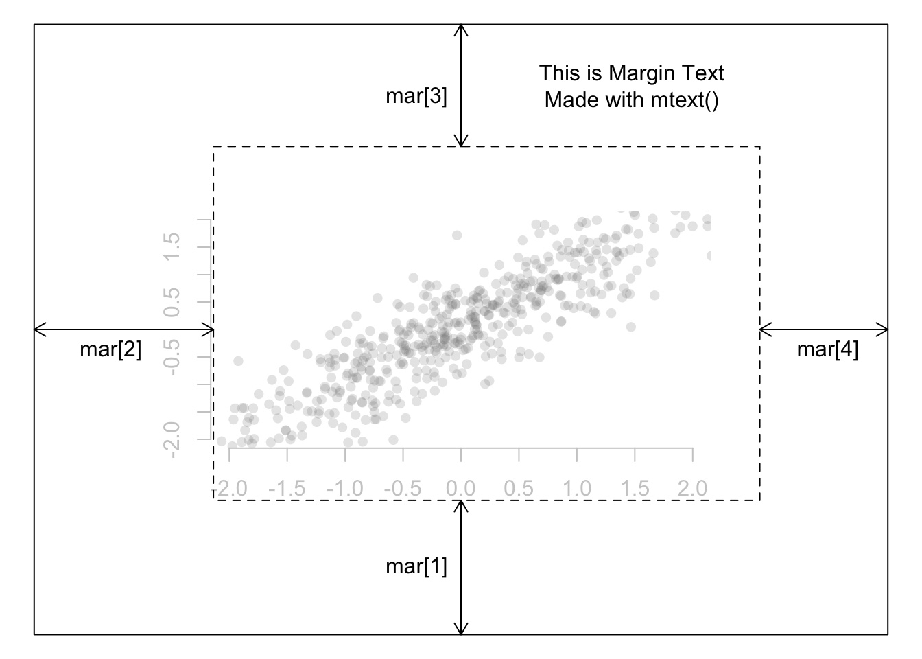
9 Margins

Maps are often stuffed full of information and expanding the margins might be one strategy for improving the map’s aesthetics/usefulness. In the base plot parameters, the par(mar = c(5, 4, 4, 4) + .01) is the function. The numbers specify the number of lines of margin to add on the four sides of the plot. Argument values to mar go in the following order: bottom, left, top, right. Or to help myself remember it, I use the mnemonic bacon, lettuce, tomato on rye to help remember the order. (For those more comfortable in working in inches, look for the mai argument under the help menu.)

Figure 7: Image showing the approximate default margins given to a plot (phillips2017yarrr?).

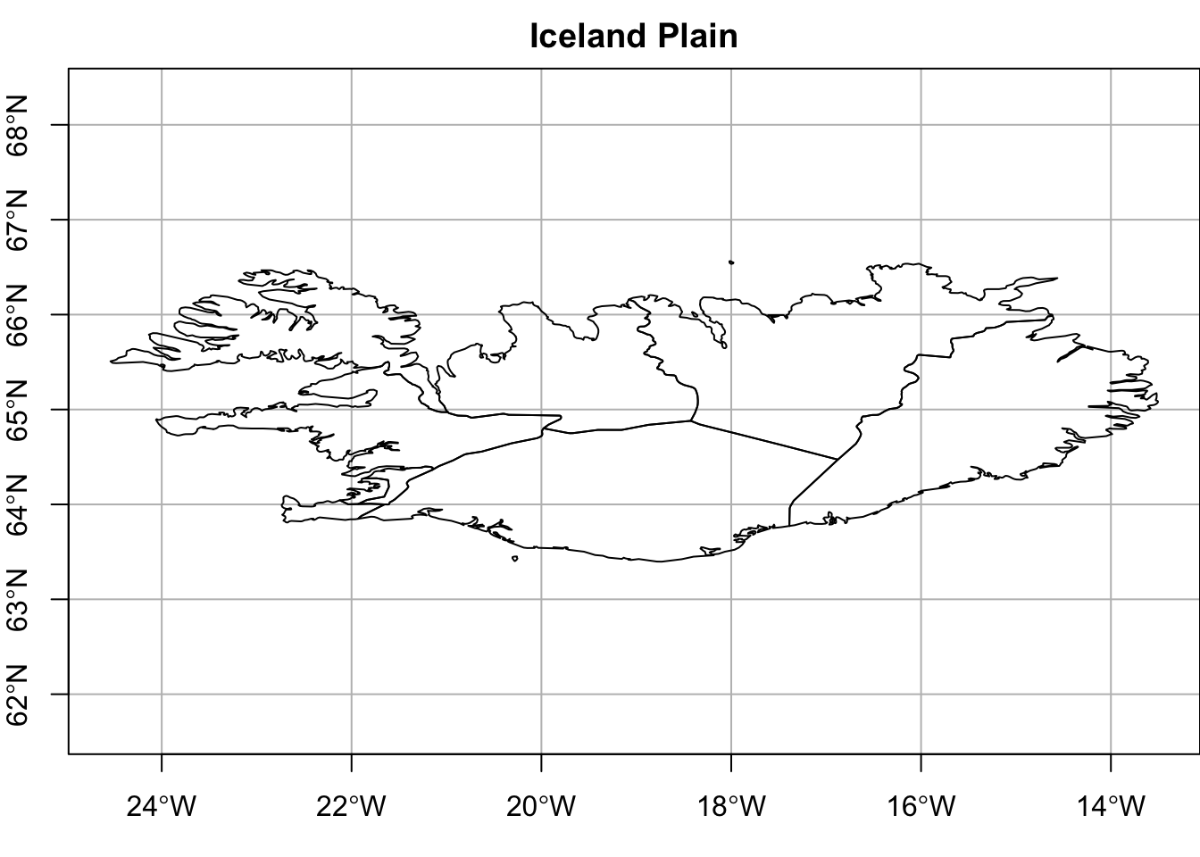
Revisiting the plain Iceland plot, we’ll show it with the default margin.

withr::with_par(list(mar = c(5, 4, 4, 2) + .1),
    plot(st_geometry(iceland),
         axes = T,
         main = "Iceland Plain",
         graticule = T,
         asp = 1)
)

1

These are the margin defaults.

2

Graticule was added.

3

Aspect ratio changed to 1 to prevent y-axis labels from overlapping. This results in a plate carrée or flat map.

Figure 8: Plot with margins expanded by two lines on each side.

withr::with_par(list(mar = c(5, 4, 4, 2) - 2),
plot(st_geometry(iceland),
     axes = T,
     graticule = T,
     main = "Iceland Plain",
     asp = 1)
)

Figure 9: Plot with right margin set to 0.

10 Key Points

• Know the class of the object: is it “sf”, “sfc” or “sfg?
• Know where to look for help.
• Make sure reset = FALSE on the first plot and add = TRUE on additional layers.
• Understand that the ellipsis ... in the help menu gives you access to additional arguments in the base ploting package.
• Reset par() options by restarting the graphics device or avoid changing them all together with the withr::with_par() function.
• Use mfrow or mfcol for multiple plots on the same page.
• Use par(mar = c("b", "l", "t", "r") to adjust margins.

---

Pebesma, E., & Bivand, R. (2023). Spatial data science: With applications in R. Chapman and Hall/CRC. https://r-spatial.org/book/