tmap
1 Objectives
The objective for this section is to introduce the tmap functions for plotting spatial data.
2 Introduction
According to the tmap website, it is used for drawing thematic maps and is based on “A Layered Grammar of Graphics” like ggplot2. (Tennekes, 2018). “A grammar provides a strong foundation for understanding a diverse range of graphics. A grammar may also help guide us on what a well-formed or correct graphic looks like . . .” (Wickham, 2010) Layers are added using the + operator just like in ggplot2. Most functions begin with the tm_ prefix. A great introduction is the package’s getting started vignette. The vignette can be seen with the following code: vignette("tmap-getstarted", package = "tmap"). With tmap you can view the map in either static or interactive mode. We’ll take up interactive plots later and focus on static maps. tmap is the primary plotting package in the “Geocomputation with R” book with the rationales being:
tmap is a powerful and flexible map-making package with sensible defaults. It has a concise syntax that allows for the creation of attractive maps with minimal code which will be familiar to ggplot2 users. It also has the unique capability to generate static and interactive maps using the same code via tmap_mode(). Finally, it accepts a wider range of spatial classes (including sf and terra objects) than alternatives such as ggplot2. (lovelace2019geocomputation?)
We’ll begin with a simple square and then move to an example of multiple squares.
These lessons were built with the development version of tmap which is moving from version 3 to 4. See the GitHub repo for latest development version and installation instructions.
3 Packages Required
4 First Plot - Square
4.1 Create Object
To get started, a square polygon will be created at the (0, 0), the intersection of the Prime Meridian and the Equator. Each side will be one unit in length and because the CRS “WGS 84” will be assigned, that unit is a degree.
4.2 Mode
tmap has two modes: “plot” and “view”. The “plot” mode is for static plots and the “view” mode is for interactive plots. The default is “plot”.
4.3 Plot
4.4 Style / Theme
As opposed to ggplot2 where a set of formats is called a “theme”, in tmap, they are called a “style”. You can see the styles available by running:
tmap::tmap_style()
#> current tmap style is ""white" (tmap default)
#> other available styles are: "gray", "natural", "cobalt", "albatross", "beaver", "bw", "classic", "watercolor"
#> tmap v3 styles: "v3" (tmap v3 default), "gray_v3", "natural_v3", "cobalt_v3", "albatross_v3", "beaver_v3", "bw_v3", "classic_v3", "watercolor_v3"
A style can be set for the duration of the programming session via tmap_style("<style>"). Note the difference between tmap_style() and tm_style().
see_tmap <- function(style){
    (square |>
    tm_shape() +
    tm_polygons() +
    tm_style(style))
}

theme_1 <- see_tmap(style = "white")
theme_2 <- see_tmap(style = "classic")
theme_3 <- see_tmap(style = "albatross")
theme_4 <- see_tmap(style = "cobalt")
theme_5 <- see_tmap(style = "watercolor_v3")
theme_6 <- see_tmap(style = "gray")

tmap_arrange(theme_1, theme_2, theme_3, theme_4, theme_5, theme_6, ncol = 3)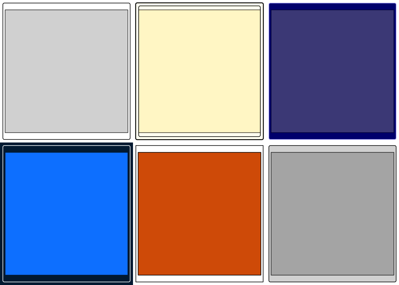
tmap using different styles.
4.5 Layering
Like ggplot2, tmap creates plots by layering geoms on the base plot using the + operator. As an illustration, a set of simple features will be created to mimic a typical map: a country, a boundary, and three cities. The name of the country is “Square” and it has three cities: “a”, “b”, and “c”.
library(ggplot2)
sf::st_polygon(list(rbind(c(0,0), c(0,1), c(1,1),
                          c(1,0),  c(0,0)))) %>%
st_sfc(., crs = 4326) %>%
st_sf(name = "Square", geometry = .) -> country

country %>% st_boundary(.) -> boundary

st_sfc(st_point(c(.5, .1)),
       st_point(c(.8, .9)),
       st_point(c(.2, .4)),
       crs = 4326) %>%
st_sf(name = letters[1:3], .) -> cities

country %>% st_centroid(.) -> centertmap_mode("plot")
tmap_style("white")
p1 <- tm_shape(country) + tm_polygons(fill = "white")
p2 <- tm_shape(country) + tm_polygons(fill = "antiquewhite")
p3 <- tm_shape(country) + tm_polygons(fill = "antiquewhite", lwd = 4)
p4 <- p3 + tm_shape(cities) + tm_dots(col = "black", size = .5)
p5 <- p4 + tm_shape(cities) + tm_text("name", col = "black", size = 1.25, xmod = -1)
p6 <- p5 + tm_shape(center) + tm_text("name", size = 1.5)
p7 <- p6 + tm_layout(bg.color = "skyblue")
tmap_arrange(p1, p2, p3, p4, p5, p6, p7, ncol = 3)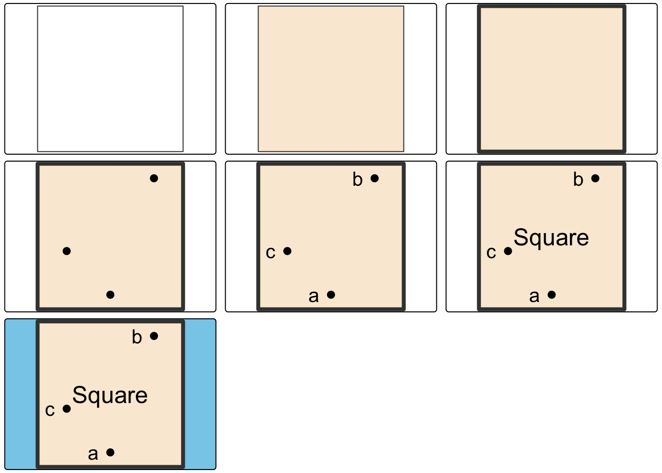
5 Second Plot - Square Land
5.1 Create
Like the ggplot2 example, this second example will begin to resemble an actual map. First, Africa will be added as a base layer via the rnaturalearth package. Then, two sf class squares will be created. These squares/islands are around the intersection of the Equator and the Prime Meridian. Then, a mountain, a lake, the Equator and Prime Meridian will be added along with the accompanying text and labels. Finally, the background will be colored blue to resemble water.
afrc <- rnaturalearth::ne_countries(continent = "Africa")

# create simple features
land_1 <- st_polygon(list(rbind(c(-10, -10), c(-10, -15), c(-15, -15), c(-15, -10), c(-10, -10))))
land_2 <- land_1 * .75 + 7
lake <- land_1 * .25
mountain <- st_centroid(land_1 - 1)
pm <- st_linestring(matrix(c(0, -20, 0, 20), ncol = 2, byrow = T))
eq <- st_linestring(matrix(c(-20, 0, 20, 0), ncol = 2, byrow = T))

# sfc
land_sfc = st_sfc(list(land_1, land_2))
lake_sfc = st_sfc(lake)
mountain_sfc <- st_sfc(mountain)
pm_sfc <- st_sfc(pm)
eq_sfc <- st_sfc(eq)

# set CRS
land_sfc_wgs = st_sfc(land_sfc, crs = "OGC:CRS84")
lake_sfc_wgs = st_sfc(lake_sfc, crs = "OGC:CRS84")
mountain_sfc_wgs <- st_sfc(mountain_sfc, crs = "OGC:CRS84")
pm_sfc_wgs <- st_sfc(pm_sfc, crs = "OGC:CRS84")
eq_sfc_wgs <- st_sfc(eq_sfc, crs = "OGC:CRS84")

# add attributes
country <- c("A", "B")
land_sfc_wgs_df = st_sf(country = country, land_sfc_wgs)
name <- "Mt. High"
mountain_sfc_wgs_df = st_sf(name = name, mountain_sfc_wgs)
name <- "Lake Clear"
lake_sfc_wgs_df <- st_sf(name = name, lake_sfc_wgs)
name <- "Equator"
eq_sfc_wgs_df <- st_sf(name = name, eq_sfc_wgs)
name <- "Prime Meridian"
pm_sfc_wgs_df <- st_sf(name = name, pm_sfc_wgs)
5.2 Plot
From the length of the code below, you can see that creating and plotting maps can be a lengthy and tedious process. Label/text placement can take a lot of time. While there are some improvements to be made, I think the plot encapsulates the process and gives you a strategy to plot your own. You’ll notice that this code is not any shorter than the code in the ggplot2 code.
# identify bb in narrative
library(tmap)
library(tmaptools)
tmap_options_reset()
afrc <- rnaturalearth::ne_countries(continent = "Africa")
box <- tmaptools::bb(afrc, xlim = c(-20, 15), ylim = c(-20, 10))
afrc <- afrc[-which(sf::st_is_valid(afrc) == FALSE), ]
squareland <-
    tm_shape(afrc,  bb = box) +
        tm_polygons(fill = "antiquewhite") +
        tm_borders(col = "gray50", lwd = .25) +
    tm_shape(land_sfc_wgs_df) +
        tm_borders("gray50", lwd = .25) +
        tm_polygons("country", fill = "antiquewhite") +
        tm_text("country", ymod = 1) +
    tm_shape(lake_sfc_wgs) +
        tm_polygons(fill = "lightblue") +
        tm_text("Lake Clear", ymod = -1.3, xmod =-1) +
    tm_shape(mountain_sfc_wgs_df) +
        tm_symbols(size = 1, fill = "red", shape = 17) +
        tm_text("Mt. High", ymod = -.75, xmod = 1) +
    tm_shape(eq_sfc_wgs_df) +
        tm_lines(lty = "dotted") +
        tm_text("Equator", xmod = -15, ymod = .5, fontface = "italic", alpha = .5, size = .75) +
    tm_shape(pm_sfc_wgs_df) +
        tm_lines(lty = "dotted") +
        tm_text("Prime Meridian", ymod = -14, xmod = -.5, fontface = "italic",
                alpha = .5, size = .75, angle = 90) +
    tm_xlab("Longitude") +
    tm_ylab("Latitude", rotation = 90) +
    tm_grid(labels.show = T,  alpha = .5, labels.size = .7) +
    tm_compass(position = c(.75, .25)) +
    tm_scalebar(breaks = c(0, 200, 400, 600, 800),
                position = c(.65, .1)) +
    tm_title_in("Square Land",
                size = 1.4,
                padding = c(.5, 1, .5, 1),
                position = tm_pos_in("left", "top"),
                bg.color = "white",
                frame = "black",
                frame.lwd = 2) +
    tm_layout(
              bg.color = "lightblue",
              inner.margins = 0,
              frame = "grey50",
              frame.lwd = 3,
              frame.double.line = F,
              outer.bg.color = "#00000000"
              )
squareland
tmap
6 Key Points
tmapsyntax is similar toggplot2tmaphas two modes: “plot” and “view”Use
tmap_style()to set the style of the plotLayers usually begin with a call to
tm_shape()