Square Land

1 Objectives

The objective for this section is to introduce the ggplot2 functions for plotting spatial data.

2 Introduction

The ggplot2 package is the default plotting package for most R users. The key functions are geom_sf and coord_sf. A close reading of the help menu can speed the generation of plots. For those in a hurry, I’d recommend Chapter 6 “Maps” in “ggplot2: Elegant Graphics for Data Analysis (3e)” by Hadley Wickham (Wickham, 2016). We’ll begin with a simple square and then move to an example of multiple squares.

3 Packages Required

library(cowplot)
library(ggplot2)
library(ggspatial)
library(magrittr)
library(patchwork)
library(sf)

4 First Plot - Square

Let’s create as simple an object as possible so that we can focus on the syntax; repeat some of the sf functions and the sfg >> sfc >> sf pipeline; and show the multiple ways that ggplot2 syntax can result in a plot.

4.1 Create Object

To get started, a square polygon will be created at the (0, 0), the intersection of the Prime Meridian and the Equator. Each side will be one unit in length and because the CRS “WGS 84 / 4326” will be assigned, that unit is a degree.

sf::st_polygon(list(rbind(c(0,0), c(0,1), c(1,1), 
                          c(1,0), c(0,0)))) %>%
st_sfc(., crs = 4326) %>%
st_sf(name = "square", .) -> square

4.2 Syntax

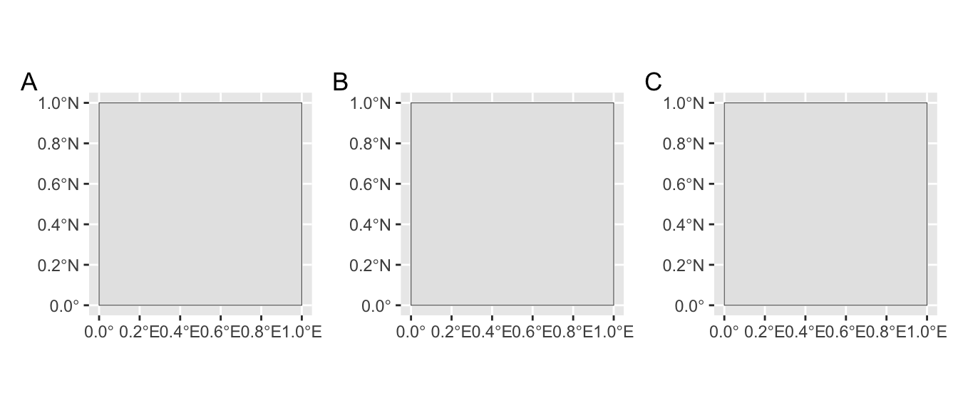
The three plots are put side-by-side to show that while the syntax changes, the output does not. You can expect the syntax to change throughout the discussion.

square |>
ggplot() +
geom_sf() -> p1

ggplot(square) +
geom_sf() -> p2

ggplot() +
geom_sf(data = square)  -> p3

p1 + p2 + p3 + plot_annotation(tag_levels = "A")

1

A plot where the dataset is “piped” into the gglot() function.

2

A plot where the dataset is within the ggplot() call.

3

A plot where the datset is included within the geom_sf().

4

The three plots were saved and then placed on a grid using the patchwork package.

Figure 1: Simple Square Polygon. Parts (1) - (3) show that the same syntax results in the identical plot.

Terrific! With a minimal effort, a plot was generated using ggplot2. I know it doesn’t look like much, but don’t worry, we’ll continue to improve upon it.

4.3 Layering

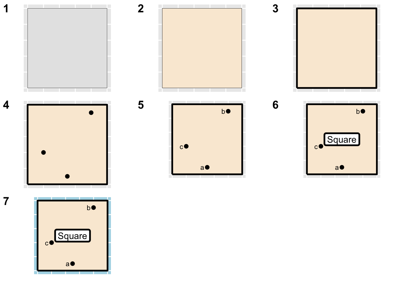
Plots and maps are created by layer. It is useful to think about the order in which they will be drawn. There are as many layers as there are potential datasets. At some point, the map becomes so jumbled that adding an additional layer is not possible and certainly not attractive. Here, is a basic illustration.

library(ggplot2)
sf::st_polygon(list(rbind(c(0,0), c(0,1), c(1,1),
                          c(1,0),  c(0,0)))) %>%
st_sfc(., crs = 4326) %>%
st_sf(name = "Square", geometry = .) -> country

country %>% st_boundary(.) -> boundary

st_sfc(st_point(c(.5, .1)),
       st_point(c(.8, .9)), 
       st_point(c(.2, .4)), 
       crs = 4326) %>% 
st_sf(name = letters[1:3], .) -> cities

country %>% st_centroid(.) -> center

ggplot() +
geom_sf(data = country) +
coord_sf(label_axes = "----") -> layer_1
layer_1 + geom_sf(data = country, fill = "antiquewhite") +
coord_sf(label_axes = "----") -> layer_2
layer_2 + geom_sf(data = boundary, lwd = 1) +
coord_sf(label_axes = "----") -> layer_3
layer_3 + geom_sf(data = cities, size = 2) +
coord_sf(label_axes = "----") -> layer_4
layer_4 + geom_sf_text(data = cities, 
                 mapping = aes(label = name), 
                 nudge_x = -.07, 
                 size = 3) +
coord_sf(label_axes = "----") +
labs(x = "", y = "") -> layer_5
layer_5 + geom_sf_label(data = center, 
                  mapping = aes(label = name), 
                  size = 4,
                  label.size = 1) +
    coord_sf(label_axes = "----") -> layer_6
layer_6 + 
    coord_sf(label_axes = "----") +
    theme(panel.background = element_rect(fill = "lightblue")) -> layer_7

cowplot::plot_grid(
    layer_1, layer_2, layer_3, layer_4, layer_5,
    layer_6, layer_7,
    nrow = 3,
    ncol = 3,
    labels = 1:7
    )
# (layer_1 + layer_2 + layer_3) /
# (layer_4 + layer_5 + layer_6) /
# (layer_7 + plot_spacer() + plot_spacer())

1

A square polygon created and assigned to variable country.

2

The boundary is created from the country.

3

Three random points are created and assigned to variable cities.

4

Center of country is calculated for label placement.

5

Seven layers are created.

Figure 2: Map creation through layering. In order, the parts are (1) base plot initiated, (2) polygon filled, (3) border added, (4) cities added (5) cities labelled, (6) country labeled, and (7) background colored light blue to resemble water.

4.4 Themes

Themes are a great way to quickly spruce up a plot and ggplot2 offers quite a few of them. You can learn more by checking help ?ggplot2::themes. I prefer to use minimal ornamentation and you’ll find the theme_void() can be helpful when assembling plots in a grid.

square %>%
ggplot() +
geom_sf(fill = "antiquewhite") +
coord_sf(label_axes = "----") +
scale_x_continuous(limits = c(-.5, 1.5)) +
scale_y_continuous(limits = c(-.5, 1.5)) -> square_map

square_map + theme_void()    -> theme_1
square_map + theme_minimal() -> theme_2
square_map + theme_bw()      -> theme_3
square_map + theme_light()   -> theme_4

plot_grid(theme_1, theme_2, theme_3, theme_4,
          nrow = 2, labels = 1:4)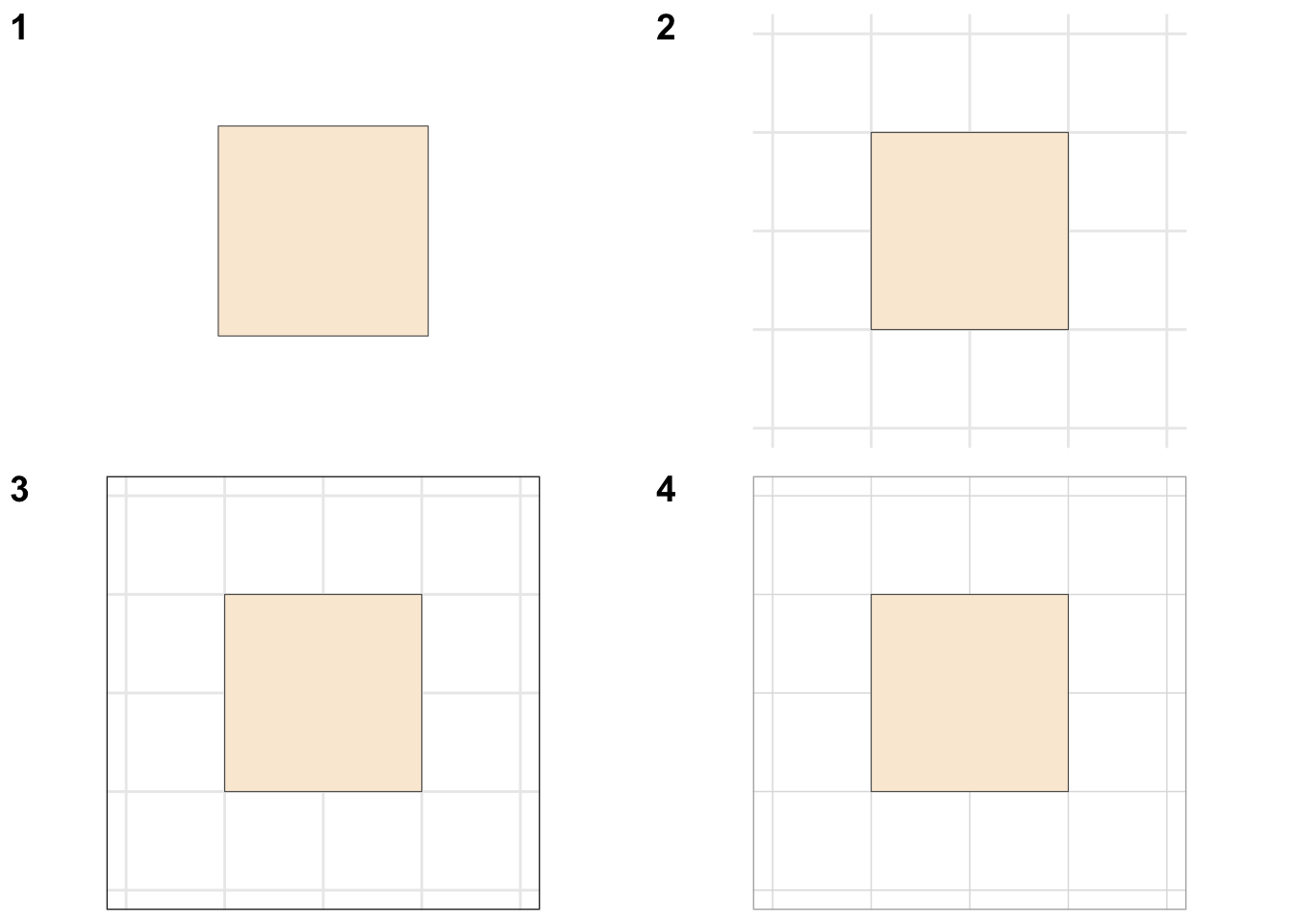

Figure 3: A polygon in four themes: (1) theme void(), (2) theme minimal(), (3) theme_bw(), and (4) theme_light().

5 Second Plot - Square Land

We’ll create Square Land features and then plot them.

5.1 Create

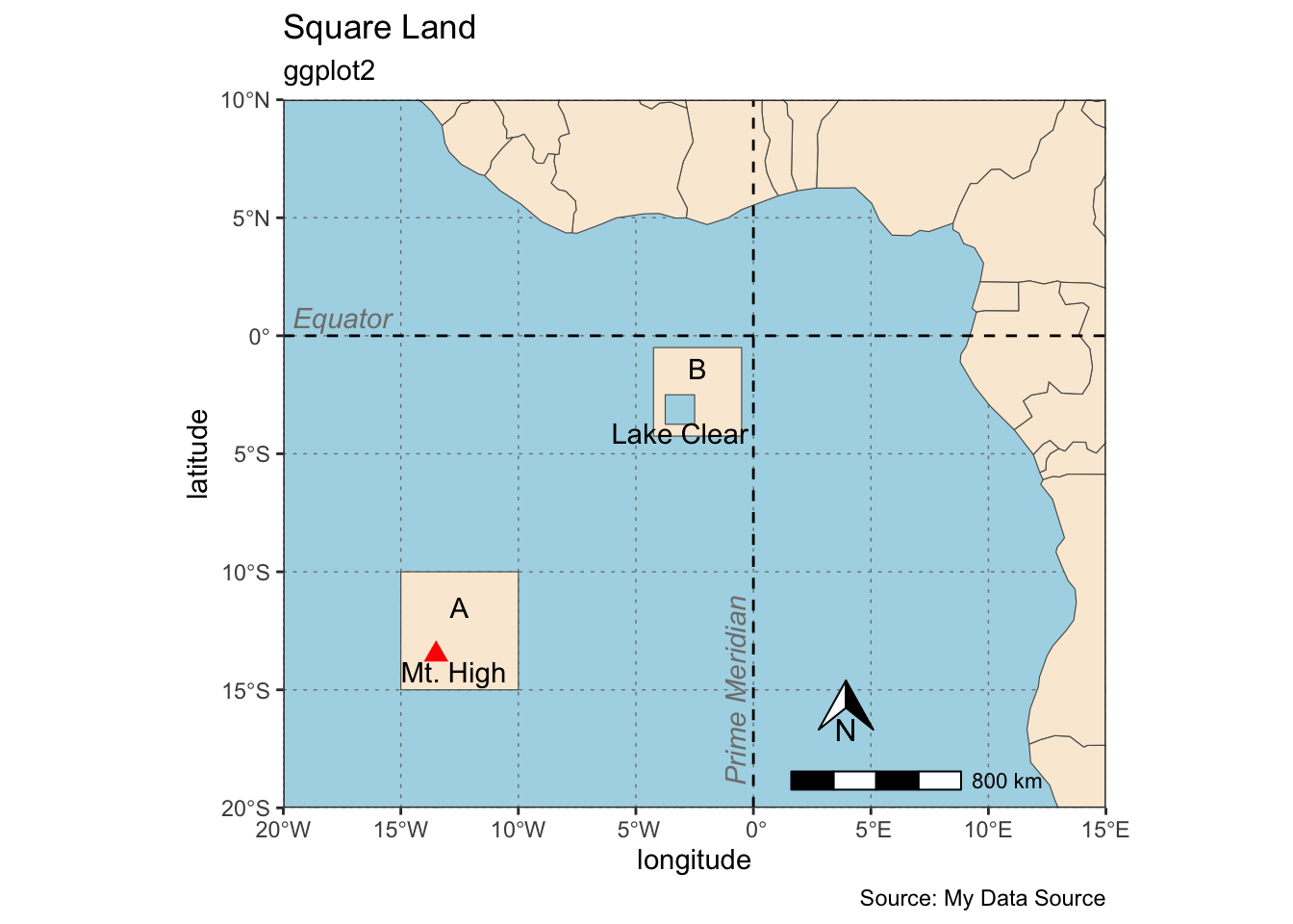
This second example will begin to resemble an actual map. First, Africa will be added as a base layer via the rnaturalearth package. Then, two sf class squares will be created. These will be squares again around the intersection of the Equator and the Prime Meridian. Then, a mountain, a lake, the Equator and Prime Meridian will be added along with the accompanying text and labels. Finally, the background will be colored blue to resemble water.

afrc <- rnaturalearth::ne_countries(continent = "Africa")

land_1 <- st_polygon(list(rbind(
    c(-10, -10), c(-10, -15), c(-15, -15), 
    c(-15, -10), c(-10, -10)))) 
land_2 <- land_1 * .75 + 7
lake <- land_1 * .25
mountain <- st_centroid(land_1 - 1)
pm <- st_linestring(matrix(c(0, -20, 0, 20), ncol = 2, byrow = T))
eq <- st_linestring(matrix(c(-20, 0, 20, 0), ncol = 2, byrow = T))


land_sfc = st_sfc(list(land_1, land_2))
lake_sfc = st_sfc(lake)
mountain_sfc <- st_sfc(mountain)
pm_sfc <- st_sfc(pm)
eq_sfc <- st_sfc(eq)



land_sfc_wgs = st_sfc(land_sfc, crs = "OGC:CRS84")
lake_sfc_wgs = st_sfc(lake_sfc, crs = "OGC:CRS84")
mountain_sfc_wgs <- st_sfc(mountain_sfc, crs = "OGC:CRS84")
pm_sfc_wgs <- st_sfc(pm_sfc, crs = "OGC:CRS84")
eq_sfc_wgs <- st_sfc(eq_sfc, crs = "OGC:CRS84")


country <- c("A", "B")
land_sfc_wgs_df = st_sf(country = country, land_sfc_wgs)
name <- "Mt. High"
mountain_sfc_wgs_df = st_sf(name = name, mountain_sfc_wgs)
name <- "Lake Clear"
lake_sfc_wgs_df <- st_sf(name = name, lake_sfc_wgs)
name <- "Equator"
eq_sfc_wgs_df <- st_sf(name = name, eq_sfc_wgs)
name <- "Prime Meridian"
pm_sfc_wgs_df <- st_sf(name = name, pm_sfc_wgs)

1

Add the base layer Africa.

2

Create simple features of sfg class

3

Combine some shapes and convert all to sfc class.

4

Assign CRS.

5

Add attributes/labels and convert to sf.

5.2 Plot

From the sheer length of the code below, you can see that creating and plotting maps can be a lengthy and tedious process. Label/text placement can take a lot of time. While there are some improvements to be made, I think the plot encapsulates the process and gives you a strategy to plot your own.

ggplot() +
geom_sf(data = afrc, fill = "antiquewhite") +
geom_sf(data = land_sfc_wgs_df, fill = "antiquewhite") +
geom_sf(data = lake_sfc_wgs_df, fill = "lightblue") +
geom_sf(data = mountain_sfc_wgs_df, 
        color = "red", shape = 17, size = 3) +
geom_sf(data = pm_sfc_wgs_df, linetype = "dashed") +
geom_sf(data = eq_sfc_wgs_df, linetype = "dashed") +
geom_sf_text(data = land_sfc_wgs_df,
             aes(label = country),
             nudge_y = 1) + 
geom_sf_text(data = mountain_sfc_wgs_df,
             aes(label = name),
             nudge_y = -.75,
             nudge_x = .75) +
geom_sf_text(data = lake_sfc_wgs_df,
             aes(label = name),
             nudge_y = -1) +
geom_sf_text(data = eq_sfc_wgs_df,
             aes(label = name),
             nudge_y = .75,
             nudge_x = 2.5,
             color = "gray50",
             fontface = "italic") +
annotate(geom = "text", x = -.75, y = -15, label = "Prime Meridian",
         fontface = "italic", color = "grey50", angle = 90) +
coord_sf(xlim = c(-20, 15),
         ylim = c(-20, 10),
         expand = F) +
annotation_north_arrow(
    which_north = "grid",
    height = unit(.75, "cm"),
    width = unit(.75, "cm"),
    location = "br",
    pad_x = unit(3.2, "cm"),
    pad_y = unit(1, "cm")
    ) +
    annotation_scale(pad_x = unit(2.75, "in")) +
labs(title = "Square Land",
     subtitle = "ggplot2",
     x = "longitude",
     y = "latitude",
     caption = "Source: My Data Source") +
theme_bw() +
theme(panel.grid.major = element_line(
    color = gray(.5),
    linetype = "dotted",
    linewidth = 0.25),
    panel.background = element_rect(
        fill = "lightblue") 
)

1

Call ggplot.

2

Add geom_sf layers.

3

Add text/label annotations.

4

Limit window to area of interest.

5

Add directional indicator.

6

Add scale.

7

Add axis and title labels.

8

Set theme.

9

Modify theme.

Figure 4: Square Land. Combining and layering of a number of simple features to create a map. Title, Subtitle, and data source included to show presentation outside of a standing narrative text.

6 Key Points

• maps are created by layering

• ggplot2 key functions for maps are geom_sf and coord_sf

• geom_sf will use the coordinate reference system from the first layer to be plotted so long as it’s not been set with the crs argument

• ggspatial package can add a directional indicator and a scale bar

• geom_sf_text will add text to the plot for labeling features

• themes can quickly polish a plot and give it a finished look

---

Wickham, H. (2016). Getting Started with Ggplot2. In H. Wickham (Ed.), Ggplot2: Elegant Graphics for Data Analysis (pp. 11–31). Springer International Publishing. https://doi.org/10.1007/978-3-319-24277-4_2