United States
1 Objective
The objective for this section is to create a choropleth map of the 50 United States, including Hawaii and Alaska.
2 Introduction
This section describes how to build a choropleth map of the United States. The U.S. provides an excellent case study because two states – Alaska and Hawaii – are not connected to the mainland. Alaska and Hawaii are dissimilar in that Alaska is large and close to the North Pole, while Hawaii is small and near the Equator. Cartographers must resolve where to place the two states when making a map. Here, we’ll begin by creating the mainland, Alaska, and Hawaii. Then, the three objects will be placed on the same plot panel. This example relied upon the methodology in this R-spatial blog post.
tigris package
The tigris::shift_geometry() function “will shift and optionally rescale a US dataset for thematic mapping of Alaska, Hawaii, and Puerto Rico with respect to the continental United States.”(Walker, 2024) The tigris package can speed development for U.S. choropleth maps.
3 Packages Required
4 Create
Returning to the rnaturalearth package, we retain the United States of America and its subdivisions. The original dataset contains the District of Columbia which is dropped. A random variable is created and then broken into five separate groups as an ordered factor using the ggplot2::cut_interval() function.
4.1 Data
ne_states(country = 'united states of america') %>%
select(name, postal, geometry) %>%
filter(postal != "DC") %>%
mutate(cont_var = rnorm(n = 50), .before = geometry) %>%
mutate(
fact_var = cut_interval(
cont_var,
n = 5,
labels = c("very low", "low", "average",
"high", "very high" )
),
ordered_result = T
) %>%
rmapshaper::ms_simplify(method = "vis", weighting = .05) %>%
st_transform(2163) -> us
us %>% mutate(fact_var = fct_rev(fact_var)) -> us
#> ── R CMD build ─────────────────────────────────────────────────────────────────
#> * checking for file ‘/private/var/folders/hm/r4s1x8yd7t3drh0tjd1gkwl00000gn/T/RtmpXFszOR/remotesce67305d3fe3/ropensci-rnaturalearthhires-e02c28d/DESCRIPTION’ ... OK
#> * preparing ‘rnaturalearthhires’:
#> * checking DESCRIPTION meta-information ... OK
#> * checking for LF line-endings in source and make files and shell scripts
#> * checking for empty or unneeded directories
#> * building ‘rnaturalearthhires_1.0.0.9000.tar.gz’- 1
- Create random, continuous variable.
- 2
- Group continuous variable into five groups.
- 3
- Reverse the factor order so legend entries are reversed.
4.2 Mainland
With the original dataset already created, the individual states must be extracted and plotted. The largest grouping of states is the 48 contiguous states which is named “main” in the code below.
ggplot() +
geom_sf(us, mapping = aes(geometry = geometry,
fill = fact_var),
linewidth = .4,
color = "gray80") +
scale_fill_discrete_sequential(palette = "Emrld", rev = F) +
geom_sf_text(us,
mapping = aes(label = postal),
size = 3,
check_overlap = T) +
coord_sf(crs = st_crs(2163),
xlim = c(-2500000, 2500000),
ylim = c(-2300000, 730000)) +
labs(fill = "Factor") +
theme_nothing() -> main- 1
- Declare polygon fill variable.
- 2
-
Function is from the
colorspacepackage. - 3
-
Used the
check_overlapargument to clean map text. - 4
- Set window to continental U.S.
- 5
- Rename legend.
- 6
-
theme_nothing()passes clean grob to code below.
4.3 Alaska
Alaska is projected using CRS 3467 which has the nice effect of rotating it as well for the final placement.
ggplot(data = us) +
geom_sf(mapping = aes(fill = fact_var), show.legend = F) +
coord_sf(
    crs = st_crs(3467),
    xlim = c(-2400000, 1600000),
    ylim = c(200000, 2500000),
    expand = FALSE,
    datum = NA) +
scale_fill_discrete_sequential(palette = "Emrld", rev = F) +
geom_sf_text(data = us, mapping = aes(label = postal), size = 3) +
theme_nothing() -> ak
4.4 Hawaii
The same basic approach for Alaska is applied here too, with the exception of the CRS being set to 4135.
ggplot(data = us) +
geom_sf(mapping = aes(fill = fact_var), show.legend = F) +
coord_sf(crs = st_crs(4135),
         xlim = c(-161, -154),
         ylim = c(18, 23),
         expand = FALSE,
         datum = NA) +
scale_fill_discrete_sequential(palette = "Emrld", rev = F) +
geom_sf_text(data = us,
             mapping = aes(label = postal),
             size = 3,
             check_overlap = T) +
theme_nothing() -> hi
5 Choropleth
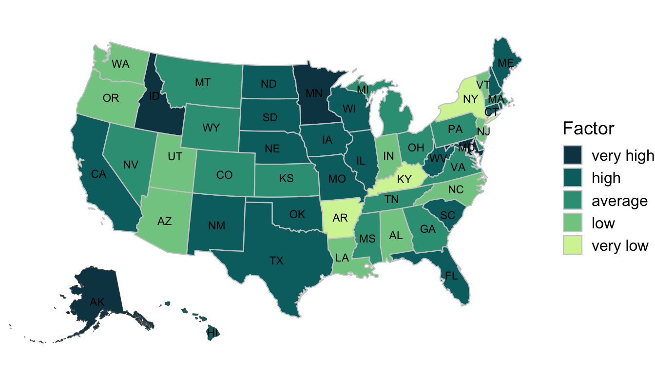
The Alaska and Hawaii grobs are placed on a panel just below and to the west of Texas. There was–and probably always is–a lot of trial and error in placing the objects on the new panel. The final tweaks were to the legend. Ultimately, the legend was left outside and to the right of the map. Note that the dark colors are for “very high” values and that the legend entries read from high to low in a downward orientation.
 main +
annotation_custom(
    grob = ggplotGrob(hi),
    xmin = -1250000,
    xmax = -1250000 + (-154 - (-161)) * 120000,
    ymin = -2450000,
    ymax = -2450000 + (23 - 18) * 120000
) +
annotation_custom(
    grob = ggplotGrob(ak),
    xmin = -2750000,
    xmax = -2750000 + (1600000 - (-2400000))/2.5,
    ymin = -2450000,
    ymax = -2450000 + (2500000 - 200000)/2.5
) +
theme_nothing() +
theme(
      legend.position = "right",
      legend.key.spacing.y = unit(2, units = "points")
      )
6 Key Points
Determine whether the areas of interest are contiguous or not
Determine the best coordinate reference system for projection
Create a separate graphical object for each non-contiguous geometry
Consider adding an annotation that warns readers that states are not to scale