New Zealand

1 Objectives

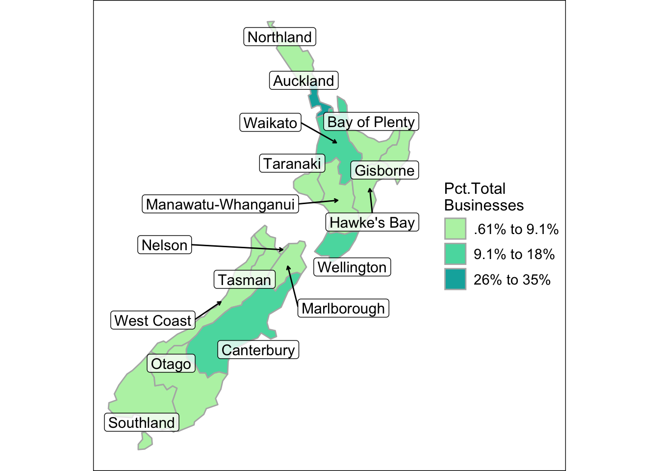
The objective in this section is to produce a choropleth map of New Zealand with ggplot2.

2 Introduction

Up until now, the ggplot2 examples were demonstrating basic principles in map building. Here, we’ll build our first real choropleth map using New Zealand as an example. We’ll go through the full production pipline by (1) importing an sf data frame, (2) cutting the variable into bins, (3) labeling the factor variable and (4) plotting multiple layers of the map.

3 Packages Required

library(colorspace)
library(dplyr)
library(ggplot2)
library(ggrepel)
library(magrittr)
library(sf)
library(tibble)
library(mapswrData)

4 Create

The first step is to load the nz_business data from the mapswrData package.

data(nz_business)
nz_business %>% st_drop_geometry() %>% slice_head(n = 5)
#>   country island      region indicator count  total pct_business lng   lat
#> 1      NZ  South   Southland   2024M04 14217 626373         2.27 168 -45.7
#> 2      NZ  South Marlborough   2024M04  7233 626373         1.15 174 -41.7
#> 3      NZ  South      Nelson   2024M04  6636 626373         1.06 173 -41.2
#> 4      NZ  South      Tasman   2024M04  7581 626373         1.21 173 -41.4
#> 5      NZ  South  West Coast   2024M04  3822 626373         0.61 171 -42.8

5 Business Indicators

The data comes from the official New Zealand Statistics agency. The metadata state that it is “a monthly count of enterprises as at the end of each month, mostly sourced from administrative data” and includes only “economically significant enterprises. It can be an individual, private-sector and public-sector enterprises.” These enterprises have a “GST turnover greater than $30,000 per year” (Stats New Zealand, 2024). The column “pct_business” will be assigned to a bin for the choropleth map.

nz_business %>% 
mutate(pct_bus_f = cut_interval(pct_business, n = 4, dig.lab = 1), 
       .before = geometry) -> nz_bus
levels(nz_bus$pct_bus_f) <- c(".61% to 9.1%",
                               "9.1% to 18%",
                               "18% to 26%",
                               "26% to 35%")

6 Choropleth

values = colorspace::sequential_hcl(4, palette = "TealGrn", rev = T)
ggplot() +
geom_sf(data = nz_bus, mapping = aes(fill = pct_bus_f), 
        lwd = .5, col = "gray70") +
scale_fill_manual(name = "Pct.Total\nBusinesses", values = values) +
geom_label_repel(data = nz_bus,
                mapping = aes(x = lng, y = lat, label = region),
                force = 10,
                fill = alpha(c("white"),0.75),
                label.padding = .2,
                box.padding = .6,
                min.segment.length = 1.2,
                arrow = arrow(length = unit(0.01, "npc"),
                              type = "open"),
                size = 4) +
theme_void() +
theme(
    legend.text = element_text(size = 11),
    legend.title = element_text(margin = margin(t = 0, r = 0, b = 4, l = 0, unit = "pt"), size = 12),
    legend.box.margin = margin(t = 0, r = 5, b = 0, l = 5, unit = "pt"),
    legend.key.spacing.x = unit(1, units = "pt"),
    legend.key.spacing.y = unit(2, units = "pt"),
    
    plot.background = element_rect(
        fill = "white",
        colour = "black",
        linewidth = .5
  )
)

1: Use rev = T to have dark color indicate high intensity.
2: Requires a lot of time for attractive labels.
3: Most changes dealt with legend appearance.

Figure 1: May 2024 New Zealand Percentage of Businesses by District. Auckland, the home of the largest city, leads with 34.7% of the nation’s businesses. Source is the New Zealand National Statistics. (If you’re from New Zealand, this may not be all that enlightening!)

7 Key Points

Geometries will often include unexpected territories and features that require design choices as to whether they should be included or omitted
Factor variables may need to be relabeled for attractive legends
The colorspace package includes a rev = argument that can be helpful in reversing the color palette
Attractive annotations in the form of labels and text are time intensive
Alter theme defaults only at the end of the project

Stats New Zealand. (2024). Enterprises Count (3ec6697f-2ec6-473b-ab41-a86e7de1fa9a). https://datainfoplus.stats.govt.nz/Item/nz.govt.stats/041540ba-fc68-4497-814a-74b2cc4beffd